To build a ML strange loop

(In the interest of exploration and trying to make it as parsable & readable as possible, this document uses various formatting options to break up the text.)

1 Synopsis

We focus on model induction for science: given data and a computatinal prior (such as a simulator), induce model(s) that best describe the data.

1. For models to serve downstream uses^§3, they ought to be in the same equivalence class as the function that originally generated the data^§4.

   • Equivalence classes are compositional, and barring mathematical transforms, two functions need to factorize in the same way to be in the same equivalence class.

2. The circuit complexity class of real-world interesting functions is \(P\), whereas most ML models are in a restricted complexity class for training or implementation reasons.

   • Therefore, to meet (1), the models need to have their complexity class promoted, while still being trainable¹¹ This problem presently garners considerable interest and effort in the field. Learnability is well respected as being difficult, and often opposed to complexity class: less complex, less capable functions are easier to learn.

3. Model induction is recursive – to solve problems, you need to induce (learn) sub-models, metrics, or conserved quantities (and their associated symmetries).

   • E.g. problems are described via validators or metrics in complexity \(P\), whereas full solution is in \(NP\). Amortization can be cast as running induced validators and algorithmically caching the results.
4. Not only should system for model induction should be re-used, independent of the level of abstraction, but the process of abstraction itself should be abstracted.

5. (3) & (4) imply setting up a strange loop[2, 3]. Current LRMs are partial strange loops; to directly represent symbolic and operational aspects of knowledge, to better execute rules of inference, and to support running algorithms from \(P\), we introduce a hypergraph transformer.

   • This is augmented with addressing^§7 & allocation^§35 extensions ¹ .

6. A model induction system needs to leverage observed symmetries and topologies in the data to factorize model structure.

   • This is akin to a perceptual system, which combats the curse of dimensionality by factorizing, reducing, and “computationalizing” the space of possible dependencies = factorizing the equivalence class.
   • Abstractions like named sets (objects) and spatial indexes (arrays) are instances of dependency elimination.
   • These abstractions themselves are computed functions, whose creation can be induced from symmetries in the data via self-supervised learning.
   • Many of these symmetries can be inferred through intervention as well (e.g. scientific method, counter-example guided synthesis).

7. In cases where information from the generating function is destroyed, aliased, unobserved²² , or unobservable³³ Including, as in (6), information about the function factorization!, even with topological perception, the system must engage amortized^§3 search or inference to derive those bits.

   • This form of analysis-by-synthesis induction must occur both during training and inference, as it does with humans.

     • Bits are bits, irrespective the timescale of their creation.

   • Inference (inversion) is very frequently acausal⁴⁴ As in the case when unobserved information affects later observations and of higher/harder complexity class than the original generating function; we can only approximate it with heuristics and rules in \(P\)⁵⁵ And thus, alas, never be in the same equivalence class.

     • Heuristics = perception here; instead of eliminating dependencies, they focus and reduce the search space.

8. To be self-organizing, the system needs to be able to perceive and act upon itself: to see and organize patterns of action and thought.

   • This means that it actively organizes its own knowledge, rather than exclusively relying on emergent organization⁶⁶ Such as through the inductive biases of SGD, or through regularization. or external supervision.

2 Historical context

Springtail was created to leverage machine learning (ML) for scientific model induction. As scientific data is often ‘expensive’, both literally and figuratively, an early focus was on sample efficiency: how do you derive the best model from limited data?

This turns out to be a very deep question, as model induction itself is (in some sense) “primal”: if you can reliably & generally solve it, you have an algorithm for understanding and operationalizing data (converting data to functions which can interpolate and (hopefully) generalize OOD). This is the whole compression-is-comprehension thesis popularized by Marcus Hutter (among others), and is perhaps why Solmonoff induction has re-emerged as a popular theme in AI startups⁷⁷ SSI, Q labs, Ndea, etc.

Initial work 2023-2024 at Springtail focused on using a generic transformer as the heuristic store (aka approximate inverse function) in DreamCoder, a landmark approach for bootstrapped program synthesis[4]. DreamCoder takes a specification, for example an image, and iteratively induces a program that can generate it. The process is inductively open-ended, so that, with increasing compute, it can solve harder and harder problems – starting from nearly zero knowledge⁸⁸ DreamCoder is given forward functions (which are certainly a form of prior knowledge) in the form of a simulator.

It didn’t work, as described in this blog post. Transformers are simultaneously too sample inefficient and don’t reliably generalize OOD in the required domain (approximate inverse graphics). We responded to this realization with an adjustment in tack, to a far simpler yet still NP-complete problem (Sudoku), ultimately leading to a highly sample efficient solver based on discrete diffusion.

Yet this still was unsatisfying, as the solver needs to see complete solutions, whereas DreamCoder was able to discover beautiful things like functional origami programming [6] de novo. What is missing? Why does the ‘weak’ (largely non-compositional) method of ProtoNets succeed where the prevalent and seemingly powerful transformer⁹⁹ Large reasoning models are architecturally just transformers fail? This instigated a deep dive into sample efficiency.

3 Sample efficiency & Generalization

Sample efficiency can be defined as the quantity of data needed to learn or induce a computational model that is quantitatively equivalent to the data, and the measurement of equivalence depends on the use of the resulting model. Equivalence and sample efficiency are usually tightly intertwined: a highly equivalent model needs fewer parameters to specify, since it does not need to ‘memorize’ (e.g. a lookup table) sub-components; in this sense equivalence is \(\propto \) compression. Often equivalence is lumped under ‘generalization’, but more explicitly includes:

• Interpolating between datapoints (kernel methods, smoothing, most neural networks)¹⁰¹⁰ Requires an ordering or metric
• Extrapolating out-of-data (OOD) or beyond supplied data (prediction, regression)
• Compression (communication)
• Disentanglement / computational gain (making downstream learning & computation easier[7])¹¹¹¹ Disentanglement can be orthogonal to compression – ideal compression maximally decorrelates and maximally packs bits into a vector = entanglement. Ideal compression also leverages a computational ‘world model’, e.g. the PAQ series of compressors
• Using the model as data itself, upstream of another algorithm (cognition) or as a description, or as a delta (as in programming)
• Using it to transform data from one domain to another (error-propagation, sorting/organizing, programming again..)

As mentioned above, model induction can hence be thought of as ‘primal’ – an essential component to any system that needs to do any (or all!) of the above. It is not usually de novo; there are always priors on the model, at minimum those imposed by the model’s substrate, which dictates what computations are possible. Ideally we have excellent sample efficiency with minimal providedpriors¹²¹² The goal is to learn those priors, and substrates with maximal generality – just like us^§14.

Machine learning is a powerful method for model induction but it is not uniformly sample efficient. Furthermore, it mostly operates with strong priors and constraints on the models & the computations that those models can do; much of the development of the field can be viewed as technological–empirical development to expand ML’s abilities in both areas¹³¹³ As mentioned in the synopsis, increasing the number and type of computations that models is often opposed to making the models easily trained. Adding constraints helps, of course. (with complementary scientific understanding often lagging behind).

In mathematics, equivalence is defined either extrinsically (by looking e.g. at set membership: if two sets have the same elements, then they are equivalent) or intrinsically (by looking at the machinery ‘within’). As induced models are typically functions and often algorithms themselves (defined over open sets), we examine intrinsic equivalence in the next section.

4 Equivalence classes

All problems can be solved via search if the solutions are recursively enumerable (countable), can be verified in finite time, and a solution exists. Model induction is in this class, where model = algorithm. Search is generally computationally inefficient, but also generally sample-efficient, and so we can start by examining the size of the search space aka hypothesis space when inducing a model from data. ¹⁴¹⁴ Equivalently: the space that must be searched to find good equivalents of the data. We will begin very general and progressively reduce the bounds.

• Models = algorithms = programs. Programs are countably infinite, \(\aleph _0\) (they are literally integers on a computer)

• The functions over integers \(i,y \in \mathbb {Z}; f(i) = y_i \) are a power set and uncountably infinite, \(2^{\aleph _0} = \aleph _1\)

  • This means that the probability of any function being computable is .. \(0\).
  • But we don’t care about that!

• To generalize OOD, two functions \(r()\) (the true function that generated the data – we assume this exists, otherwise the data is uncompressible) and \(f()\) (the function we are trying to induce / learn) must be in the same equivalence class, \( f() \in E_r \):

  \[ E_r = \{p | \forall i \in \mathbb {Z}, M(p,i) = r(i) \}\]
  where \(M\) is a Turing Machine (or, potentially, a neural network), and \(p\) are programs (or weights) that run on it.
  • As defined, the function acts upon integers, but it could be any other enumerable data.

• \(| E_r | = \aleph _0\): each equivalence class is countably infinite.

  • Trivially: by taking \(r()\) and adding any number of no-ops to it

  • Practically: \(E_r\) is a (potentially fractal & disconnected) subset of \(\mathbb {Z}\)

    • To be clear: though it’s a subset, the size is still \(\aleph _0\)!

• Rice’s theorem states that any non-trivial semantic property of a program is undecidable.

  • Determining if \(f()\) is in the same equivalence class as \(r()\) is non-trivial and therefore (theoretically) uncomputable. \(E_r\) is formally uncomputable.
  • This also means you can never be sure you have the right model: that \(f()\) \(\in E_r\) is true.

• Data is always finite, \(D = \{(x_1,y_1),(x_2,y_2), … , (x_k,y_k)\}\) and so in the real world

  \[E_r = \{p | \forall i \in \{1..k\}, M(p,x_i) = y_i \}\]

  • \(| E_r |\) is still \(\aleph _0\), alas. It does bound the number of discriminable models to \( 2^{b_D}\), where \(b_D\) is the length of \(D\) in bits.

    • This doesn’t help much: \(b_D\) is often large.
    • Even in the limit of \(k=1\), there are no restrictions: if \(f(1) = 2\) is satisfied by \(f(x) = x+x\), \(= \sqrt {x+3}\), \(= x^3 + x^2\) …
    • There must be priors over models or model classes.

• Real computation of both \(r()\) and \(f()\) is bounded in memory and time, and of limited fidelity in terms of bits or SNR. This can be expressed as a tolerance:

  \[E_r = \{p | \forall i \in \{1..k\}, | M(p,x_i) – y_i | < \epsilon _i \leq \epsilon _{all} \}\]
  Where the norm \(| |\) depends on the data, e.g. \(L_1\), \(L_2\), \(L_{\infty }\), etc.

• This finally addresses the problem: now the total number of different equivalence classes is bounded. If we define functions/programs to be the same by their equivalence class:

  \[ p_1 \sim p_2 \iff \forall i \in \{1..k\}, | M(p_1,i) – M(p_2,i) | < \epsilon _{all} \]
  Then the set of all equivalence classes is the quotient set of all programs \(P\) partitioned by \(\sim \), \((P / \sim )\), and its size is bounded
  \[| (P / \sim ) | \leq 2^{b_m}\]
  where \(b_m\) is the state-size of M as programmed by \(p_i\) (discussed more in section A.1), limited by memory and SNR.
  • Unfortunately, this relaxation also means that the ‘equivalent’ models may not extrapolate like the original generating function.
  • Humans seem to have less problem with this, hypothetically because we infer generator functions that are described by only a few functional bits and a few symmetry bits¹⁵¹⁵ And so are overwhelmingly likely in the Bayesian scheme of things. Then again, p-adic numbers….

• Composition: If \(f() \sim r()\), and \(g() \sim s()\), then \(f(g()) \sim r(s())\), where \(\sim \) is defined above. This means that equivalence classes are modular.

  • The noops mentioned above all lie in the same equivalence class, so can handily be ‘factored out’, getting closer to the Kolmogorov complexity.

  • This also means that, at the limit¹⁶¹⁶ both the limit and the Kolmogorov complexity are formally uncomputable, the compositional structure of the approximation \(f()\) must match that of the original \(r()\) for them to be in the same equivalence class.

    • What about math itself, you say? There are plenty of exact equivalences that have different compositional structures.
    • Take the Fourier transform: \(s(t) * r(t) = \mathcal {F}^{-1}(S \cdot R)\)
    • This is an application of the convolution theorem, which ‘under the hood’ involves exchanging the order and variables in the two integrals of the convolution and Fourier transform.
    • Calculus itself is a trove of equivalences that save an otherwise ‘infinite’ quantity of calculation, \(\int x \, dx = x^2 + c\), etc..
    • Most calculations have symmetries which make them invariant to reorganization or reordering (e.g. algebra);
    • Through invariances and symmetries, the tools of math can transform ‘hard’ problems of one domain into easier problems, thereby connecting otherwise disparate equivalence classes.
    • One approach to model induction would be to apply such transforms (like the Laplace transform from calculus to algebra) to make learning and induction easier.
    • Unfortunately, no one set of transformations is perfectly general. Instead, we focus on using a strange loop to learn (and learn to apply) transformations; see also ^§8

  • Wolfram is famous for emphasizing the general irreducibility of computation – which means that the equivalence class of any function (with unbounded memory and infinite SNR) is one (compositionally, excluding noops).

    • This is true, per above, but also uninteresting.
    • We, biology, evolution, even physics itself seem to care about ‘pockets’ (Wolfram’s term) of computational space that are reducible.
    • If you can’t reduce it, you can’t predict behavior without running it \(\rightarrow \) it’s unpredictable and largely useless for engineering.
    • This is true even in biology, which always ‘runs’ the system and so doesn’t need to reduce it: we have strong separation of concerns in our bodies¹⁷¹⁷ For reasons of evolvability (evolution still needs to do model induction) as well as robustness (if the system implements a different function when any of the parameters are perturbed, it cannot perform one essential task of life, which is exporting entropy to the environment).
    • In physics and mathematics we can do even better: there are multiple formulations of the same problem that are calculated in different ways. For example, Newtonian vs. Lagrangian mechanics.

• Machine learning focuses on parametric equivalence classes, which expands any given equivalence class via continuity:

  \[ E_r = \{p, \theta | \forall i \in \{1 .. k\} | M(p(\theta ),x_i) – y_i | \leq \epsilon _{all} \}\]
  \[ \theta \in \mathbb {R}^w, || \theta || \leq \epsilon _{\theta }\]
  • That is, the class is the set of programs \(p\) (often fixed by the ML researcher to one element, \(|p| = 1\)) and the set of norm-bounded \(\theta \) that ‘fits the data’.
  • Compositions of parametric equivalence classes work too, if \(f(\theta _1,) \sim r()\), and \(g(\theta _2,) \sim s()\), then \(f(\theta _1,g(\theta _2,)) \sim r(s())\). In general symmetries known to exist within the target functional representation must be introduced by the researcher.
  • Transformers are what many have realized: a means of extending the parametrically accessible set of functions to include an isolation of dependencies.

5 Equivalence classes & ML models

Most ML models are, at this point, good at interpolating data (via regularization \(+\) the inductive biases of SGD [8]); in order to satisfy further downstream uses listed in 3, we’d like them to be in the same equivalence class as the function that generated the data¹⁸¹⁸ This has degrees, of course – if the compositional structure is correct, model performance may gracefully degrade when one component does not match the original function. Also, we do not discuss noise or stochastic functions here, though they are vitally important!.

Supposition. If a ‘geometric’ functions \(r()\) is:

• Lipschitz
• Computed by continuous affine transforms (spatial warping, stretching, rotation) plus information-losing transforms (clipping, squashing)
• Without internal symmetries, or equivalently of a equivalence class that cannot be factorized
• Noiseless, or with noise that is perfectly isotropic in the output space

Then a deep MLP trained with SGD has near optimal sample efficiency approximating \(r()\), and can interpolate data perfectly¹⁹¹⁹ Yet still struggle to generalize OOD [8]. In some sense, this is just saying that the original function and the model are in the same parametric equivalence class.

For all other functions & uses, you need the function to factorize in the same way as the original function. This is where transformers come in! They start with a prior of invariance – all tokens are indistinguishable and are treated equivalently, and gradually learn functions that break this symmetry via message-passing.²⁰²⁰ Also worth noting are state-space models. Insofar as \(r()\) is a geometric function of state, these work OK. But this is a restricted parametric equivalence class.

Yet, in order to train them quickly, people normally restrict the message passing to be causal, so that nodes in the graph / tokens are not updated after they are generated. This restricts the complexity class of approximateable functions to \(TC_0\). Chain-of-thought extends this (depending on number of tokens generated) to \(NC_1\) or \(TIME\) [9, 10]; this is one way of promoting the complexity class of the model that meshes well with supervised data generated by humans. Below we outline a complementary method.

6 Hypergraph transformer

Pure functions can be expressed as a messages on a directed acyclic graph (DAG); creating models can be cast as creating, modifying, or destroying parts of this graph. Typical transformers ²¹²¹ Graph transformers that represent edges between pairs of tokens. rely on correlations within the latent space of pairs of tokens for materializing this graph in the attention matrices. Converting correlations into attention logits is mediated by the structure of the \(Q\) and \(K\) projection matrices per head, hence executable knowledge is primarily represented in the weights. Callable, abstract algorithms can be emergently learned from correlations in the training data, but they are not first-class citizens to the modelling substrate.

As outlined in ^§9.1, in order to implement flexible domain-specific rules of inference (evinced as graph operations), the model needs to be able to represent executable, actionable knowledge in rapidly modifiable memory. Insofar as message passing over a graph can implement algorithms (here of reduced complexity class), this means that you need tokens to directly modify and change this graph. Put another way, if computation can be described by a graph, then changes to this computation can be described by a hypergraph. Hence, a hypergraph transformer, which supports interactions between three tokens. Three-way interactions allows patterns between two tokens to affect the latent space of a third token (‘detect edge’), or for information in one token be sent to two other tokens (‘form edge’).

This comes at significant cost, though: \(O(n^3)\) multiplies, and \(O(n^3)\) memory, where \(n\) is the sequence length. We have reduced the memory requirement to \(O(n)\) using FlashAttention style blocking and streaming; see att3ntion git repo. Briefly, instead of a query and key, we have three tokens q, r, s that interact to form an attention tensor \(A\):

While dot product attention measures the cosine of the angle between vectors, this form of attention is the Hadamard product \((Q \odot R) \cdot S = Q \cdot (R \odot S) = (Q \odot S) \cdot R\) and does not have a intuitive geometric interpretation. Value propagation from this attention can be composed from gather and scatter operations, where gather means two tokens to one, and scatter the opposite. Gather equations:

Where \(\diamond \) is either \(+\) or (preferably) \(*\). Scatter equations:

The output is just the sum of these terms:

Further exposition is in the linked repository, which is in continued development to saturate the tensor cores & maximize FLOP throughput. In the future we may experiment with even higher degrees of between-token interaction, provided the tokens can be sorted to reduce \(n\) or the span of possible interactions²²²² This is akin to the topological organization of the cortex; dendrites support seemingly arbitrary levels of nonlinear interaction between signals, albeit over constrained input groups.

6.1 Comparisons

To compare the hypergraph and graph transformer we devised three small test tasks that require some degree of setting up or changing a graph of dependencies. For proper apples-to-apples comparison, the only part changed in the model under test is the form of the attention – either graph (normal) attention or hypergraph attention. Causal masks are not used. AdamW is used with AMSgrad; we also tried the AdamW recipe from NanoGPT. Graycode positional encoding is used (this turns out to be slightly better than standard sinusoidal position ecoding), with random phase offset.

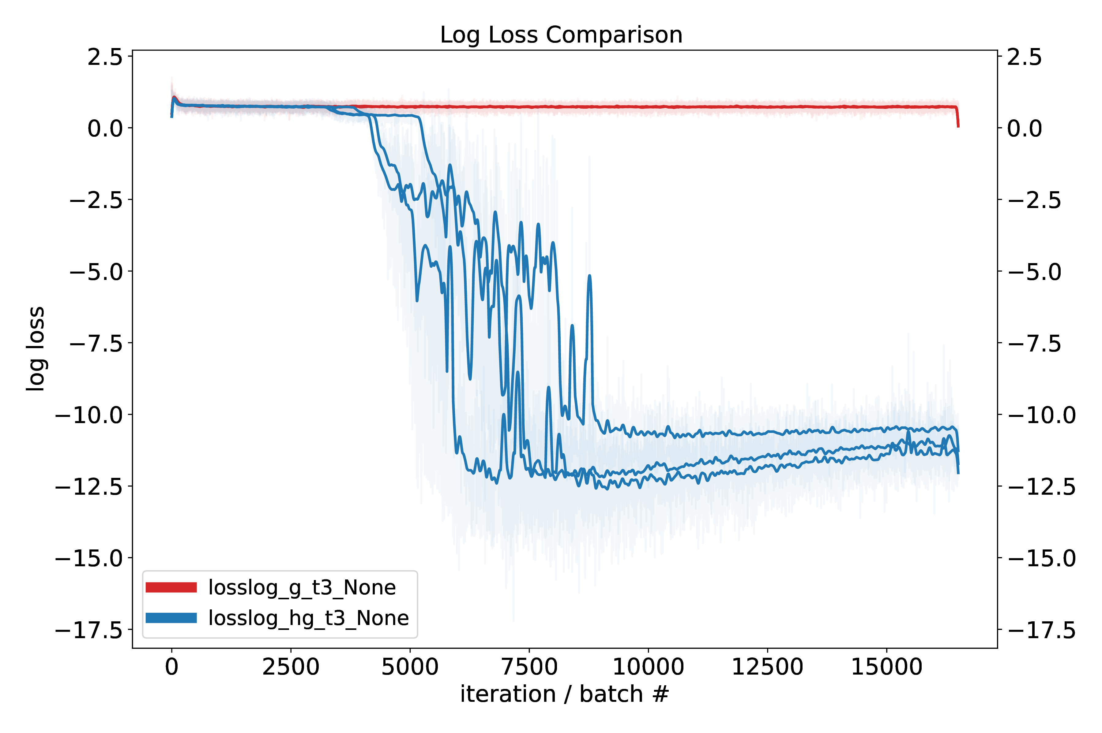
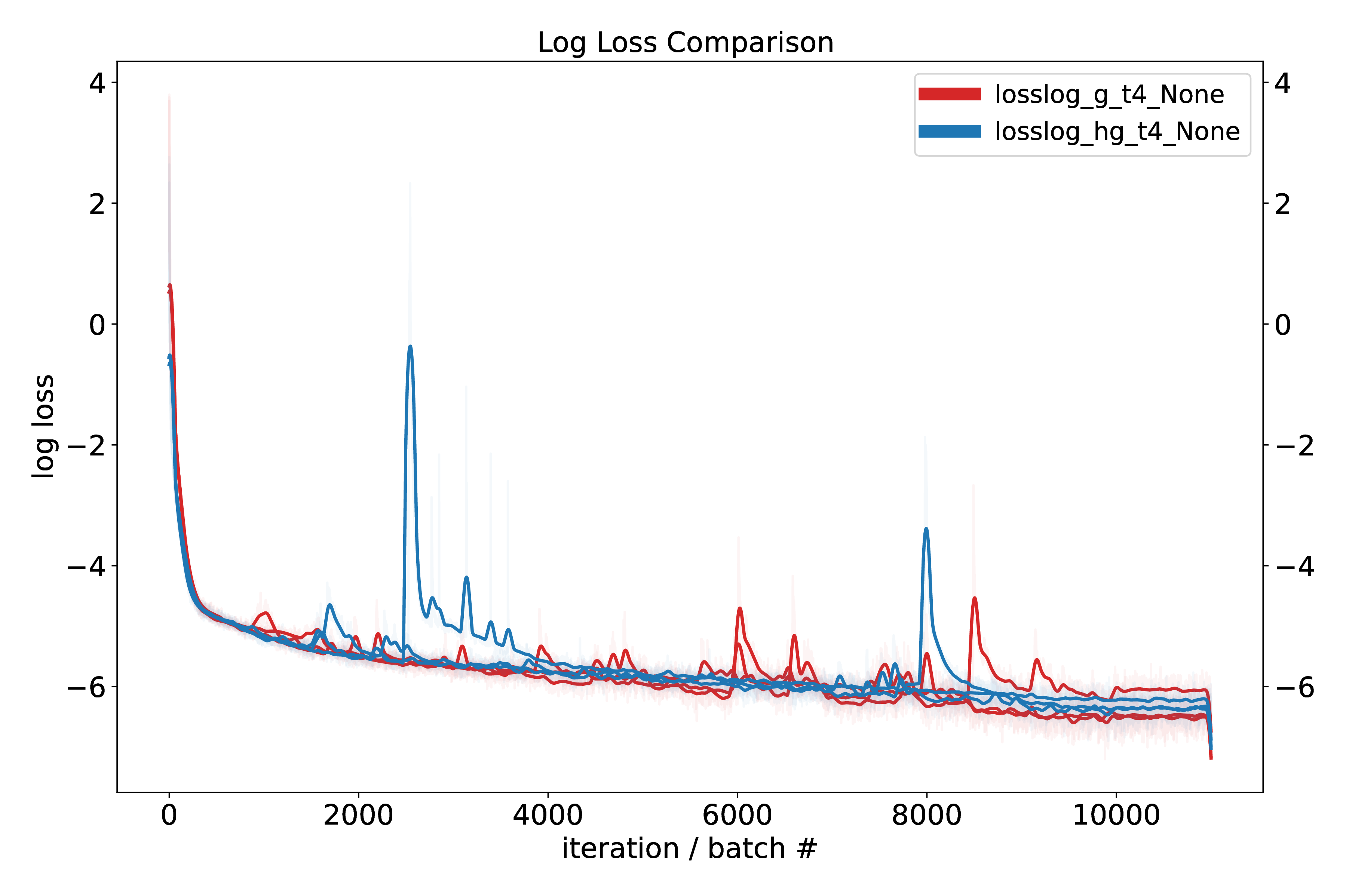
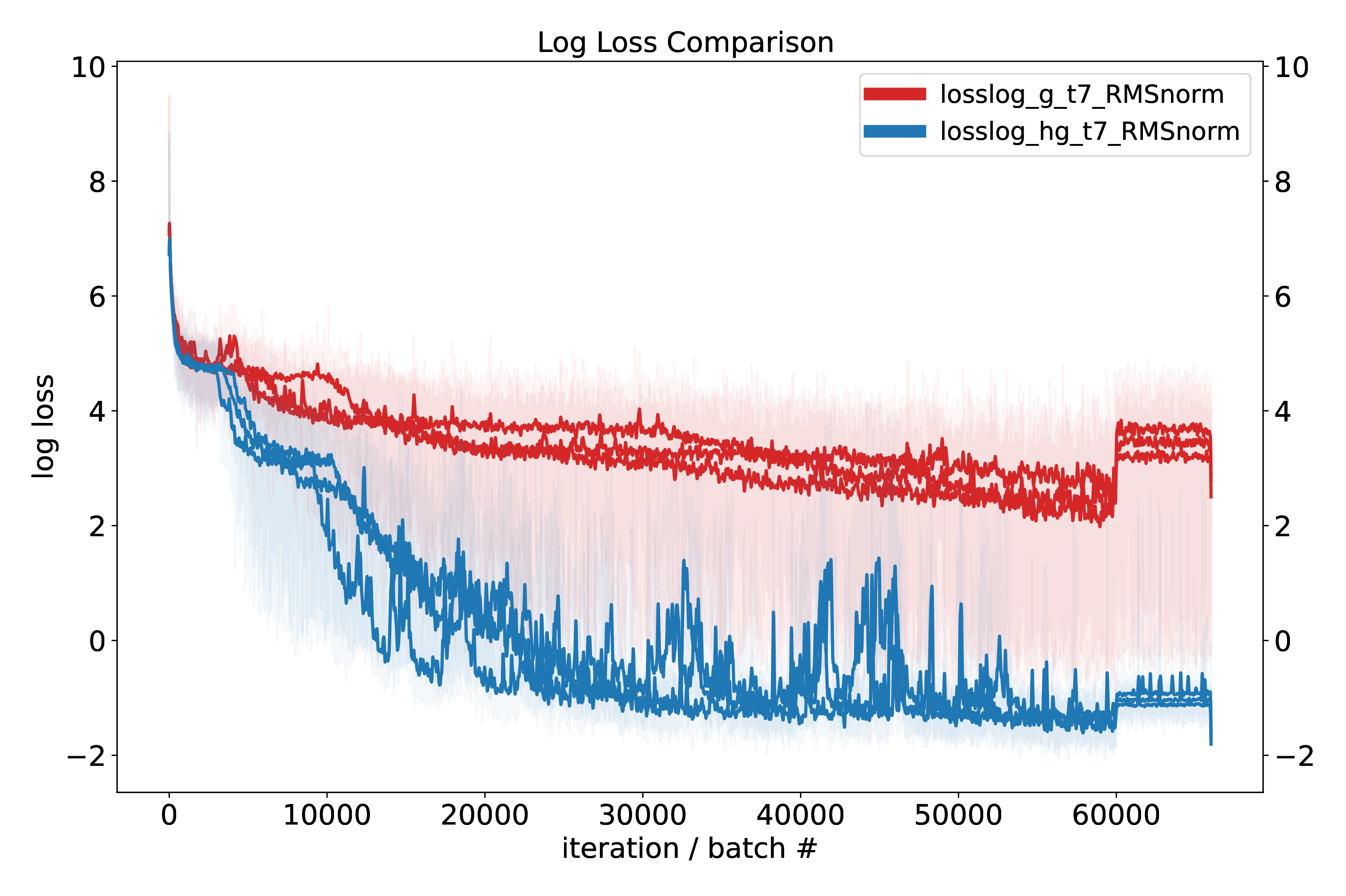
While these results are promising, we aim to perform more experiments to validate performance beyond modular arithmetic, namely on logic and reasoning tasks.

7 Extrapolation & Addressing

ML models don’t innately generalize OOD, largely due to fact that they learn Fourier features within normed spaces²³²³ Normed as in the data lies on a hypersphere, not as in a Banach space (though it’s that too). (like the Q-K space of transformers[11]), or require external supervised data to expand the envelope of probability space in un-normed spaces (like hidden layers of a MLP). Yet it is critical for science and general model-building that the resulting models do extrapolate: given a trend in the data, they reliably generate predictions, ala linear regression. Linear regression implicitly relies on the topology (ordering, distance metric, group operations of addition and subtraction) of the rationals (floats) \(\mathbb {Q}^n\), \(n \geq 1\). Likewise, classical position encoding (either RoPE or sinusoidal position encoding) relies on Fourier features to encode relative positions, which incurs some problems when e.g. asking a model to extrapolate to longer sequences than it was trained on²⁴²⁴ This is largely solved at this point. State-space models exchange this problem for others, e.g. fixed representation, different training..

The simple solution to this problem is to (continue to) exploit the built-in group operations of \(\mathbb {Q}^n\), by removing or judiciously avoiding normalization. While this has the immediate effect of reducing training stability, it doesn’t really solve the fundamental problem: the group operation in the residual stream is addition (and subtraction) on \(\mathbb {Q}^n\), whereas the addressing mesures angles, and so its operation is rotation on the hypersphere, and is hence not a group operation but rather a Lie algebra[12]. Adding to the latent stream (which in recent architectures is RMSnorm, so not mean-centered) can only increase the saturation of Softmax logits; it cannot natively shift them to different tokens.²⁵²⁵ Compare this with content – adding a vector then normalizing it makes attention Softmax-address variable content directly.

There are several options to harmonize this discrepancy. One is to adopt a form of attention that is sensitive to absolute magnitudes. \(L_1\) norm satisfies this, as is explord in this repo. It works, but suffers in training performance as:

1. The derivative is just \(\pm 1\), not the continuous magnitudes of DP attention. This makes learning harmonics on the hypersphere harder. Switching to a Huber loss adds magnitude information but in practice does not seem to help much.

2. The \(L_1\) norm is \(\ge 0\), which means that to “push up” on a given point (to select certain tokens more), all the other tokens need to be “pushed down”, which is a contrastive operation and quite slow[1]. DP attention, which is signed, does not have this problem; tokens can be enhanced and repressed freely.

   • It is also possible to use \(L_2\) norm, but we have not tried this, as the expected value of the \(L_2\) distance between points tends toward a constant as the dimensionality increases. \(L_2\) is also unsigned.

As attention is calculated between all tokens of a context, which is \(O(n^2)\) operations for graph attention and \(O(n^3)\) for hypergraph, computational expediency gives little flexibility in this calculation: it has to be simple and fast. Operations on the tokens, meanwhile, are \(O(n)\), so some complexity is tolerable. RoPE [13], SPE, CoPE [14], APE [15], FoX [16], PaTH [17] fall into this category. PaTH in particular is interesting in that it encodes information about all ordered intervals in an accumulating Householder transformation matrix, efficiently factorized for fast GPU calculation. This is halfway there; what we need is a parameterized Givens rotations to convert the latent space to rotations.

This requires matrix exponentiation (Lie algebra) or transcendental functions (\(\sin , \cos \)) based on the token contents. If you know the start and rotated vectors, as would occur in supervised learning, you can approximate a Givens rotation with a Householder reflection about a plane – but then would need to calculate \(\arcsin \) and \(\arccos \) to form a regression target for generating rotations during inference²⁶²⁶ There may be some trick here, such as using Wedge products to rotate vectors, but I don’t see it now. Some form of generator functions are required.

Separating address space and value space is a viable alternative to Givens rotations. This is typically done in programming languages, with communication between the two deliberately limited. This was done in DeBERTa [18]²⁷²⁷ It also might be similar to the apical-basal dendritic divide common in cortical pyramidal neurons: apical = feedback address calculation, basal = value calculation..

We intend to investigate both options in coming months. Addressing via spaces is a fundamental form of abstraction, and is the next abstraction operator above named variables²⁸²⁸ Which is unordered; addressing & grouping via reference; it is integral to both algorithm implementation and perceptual inference, as will be discussed in the next section.

8 Perception, symmetries, & lifting

There are many perspectives on perception: it can be cast a case of model-induction, with an emphasis on speed in exchange of approximation accuracy²⁹²⁹ I.e. the model is a scene-graph of the visual world; inference is primarily feed-forward; iterative inference only required for a few higher-level bits. If sensation is thought of as a projection, where the vast details of the world are cast down and entangled into a lower-dimensional ‘shadow’, then perception = inverse-projection. The former is a perspective of computationalism and functionalism (the model is a function or algorithm); the latter adopts the language of topology. With respect to topology, visual data famously lives on a high-dimensional manifold; prominent neuroscience theories propose that the visual cortices ‘untangle’ or ‘disentangle’ local axes of variation to separate objects from background, label objects with attributes, track continuity through time and space, etc. This is equivalent to a topological ‘lifting’ operation, where hidden axes of variation or latents are introduced to simultaneously match the projection and to satisfy observed continuity and symmetry constraints.

A symmetry is an invariance to some transformation (linear translation, rotation, scaling, reflection, cyclical or periodic translations, etc). In topology, symmetries are ‘gluing’ or division operations: space is divided up by an equivalence relation or invariance. They both hide information³⁰³⁰ e.g. gluing the real number line into a circle makes all multiples of \(\pi \) project to the same point but also reveal where nature can be cleaved at the joints; symmetries mean that some quantity is conserved, irrespective of a transformation, which directly implies invariances and equivariances in either the projection or underlying causal generative process.

Topology is also the study of continuity: quantities change at a controlled rate as you move along a surface (no change or conservation is an exemplar of this). If we make the assumption that most things change at most slowly – this means both the data and the computations that act on them³¹³¹ Making a model is just a manifestation of the assumption that the computation never changes – then symmetries frequently impose discontinuities. For example, if you glue the real line into a circle by mapping all \(2 \pi n, n \in \mathbb {Z}\) to 0, then traversing the real line results in a series of discontinuous jumps. In the case of translation, an object moving across a field of view means that a pixel abruptly and discontinuously ‘jumps’ when the projection transitions from background to object and back again. The same is true of scaling and rotation.

To resolve these discontinuities, you must induce a variables that disentangle, disambiguate, or explain the data, preferably in a way that makes trajectories smooth and continuous (if not constant). In the case of the circle, this could be an extra counter for the number of rotations around the circle. For the translation example, it’s a bit more complicated as you need a mask isolating background from object, an image of the object (like a sprite), and a translation vector \(\rightarrow \) two invariants and an equivariant. This ties well into topology: in high-dimensional pixel space, object permanence means that data is constrained to a minuscule manifold within it, with the tangent space fundamentally \(\sim 2D\). It also has a meaningful interpretation from the functional viewpoint: given a sprite, mask, and translation algorithm, all that needs to change is the translation input. Finally, this is clearly consistent with the lens of computational compression, as it reduces a complex data distribution to constants (including the computation) plus a few slowly-varying latents.

8.1 How to generate or infer these latents?

A key, I think, is that the observation of a symmetry inevitably ‘leaks’ information of one or a set of latent variables[19], and this is sufficient inductive bias for an otherwise impossible task[20]. If you’re constrained to a manifold with much smaller volume than the entire data, and the manifold is continuous, then there must be a functional way of indexing it. So, if image A predicts image B – indicating symmetry, that something is conserved – then there usually are latent or indexing variables that can transform A to B. Symmetry detection can be thought of as a (constrained) all-to-all correlation detection task, where the observed correlations are the seeds for building lifting variables. For example, you can perform unsupervised object-background image segmentation by forming a sparse affinity matrix of pixels \(W\), converting it to the graph Laplacian \(D_{ii} = \sum _j W_{ij}; L = D – W\), and taking the eigendecomposition of \(L\). The second eigenvector is then an approximate mask that cuts the similarity matrix into two regions, forming a new latent lifting variable in the same space (indexed by) the same variables used to measure the correlation – here spatial coordinates. To perform a correlation you need to have shared indexing variables = an ordered space over which to measure symmetry. This is one reason why spatial addressing^§7 is critical for chaining topologies and extraction of symmetries.

Graph-Laplacian segmentation is an explicit means of recognizing and extracting symmetries from one image; if multiple views are available, symmetries in the form of diffeomorphisms are sufficient[21]. There are likely many different instances of this form of algorithm[22]; it could also be solved implicitly by self-supervised methods[23, 24], hierarchical VAEs[25, 26] or predictive coding[27, 28, 29] networks that:

1. Perform inference to generate episodic latents; these + model structure exploit symmetries explain the data³²³² Model-based RL like EfficientZero[30, 31] is a direct inspiration, as is AXIOM[32] and the Free Transformer[33]

   • Per the argument above, the model structure should be in the same equivalence class as the original generating function.

   • Inference is performed on the generative graph via message passing ³³³³ A critical unresolved aspect is how to normalize the variables to represent probabilities.

     • Time and space can be traded off – you can infer latents through more iterations or more parallel messages. Hypothetically the visual system leans into the latter: many predictors make light work.
     • In the case that the information about latents is distributed forward in time, inference must be acausal over memory of the past.

   • If the true generating function projects \(X \rightarrow Y\), and you infer latent \(Z \approx X\), then the lifting variables need to be in the perceptual space \(Y\), not \(X\) or \(Z\)³⁴³⁴ Thanks to Henry Bigelow for this point.

     • Think the sprite example – the object mask are in the perceptual-pixel space.
     • This requires a fundamental asymmetry in the inference architecture: inference requires more variables than synthesis.
   • If transformers are used – preferred as they encapsulate lifting/abstraction via the attention mechanism^§8.1 – some of the episodic latents should be new tokens, not just new vectors of the latent space. This is the task of the aforementioned and yet-unsolved allocation module.

2. Deliberately move information about conserved computations to long-term weights.

   • Movement is controlled by the learning rate in frameworks like predictive coding, which is only the simplest form of prior, ala an exponential moving average.
   • It is possible that even this simple prior suffices when the computational graph predicting the data focuses errors to specific locations³⁵³⁵ As empirically seems to be happening in post-training frontier LLMs
   • Alternately, the strange-loop type recurrence allows the model to be its own prior.

3. Amortize the iterative inference through a parallel ‘policy’ network

   • This is like a perceptual vocabulary: you recognize & segment objects based on quick, feedforward pattern recognition modules.
   • Inferred latents are supervised targets for this amortization layer; with respect to above, this should ultimately include the supervised generation of new tokens.

With (1) you want the network to learn \(P\) functions that describe invariants in the data; this is akin to validators, constraints, or energy-based models[34]. As general perception is a \(NP\) problem, you must run some form of interative inference over the models to generate new bits to un-project or lift the perceptual shadow into a causal model. Treating the generative graph as the same as the inference graph is the perspective of analysis-by-synthesis [35], but it does not work for all problems, which is why you need a heuristic amortization layer. Building a model that does both variable-timescale Bayesian inference and fast feedforward latent prediction is a broad problem which will be the topic of the next year of research.

8.2 Interventions

Active causal intervention picks up where passive symmetry observation falls off for the inference of latents. If you push the real number wrapped to a circle example above by \(2 \pi \) and observe the no change, then the push is your exact lifting variable! Likewise, moving the eyes and head about in the world is a re-afferent signal that enables areas like the parietal cortex to learn large-scale translations of the physical world from egocentric to allocentric coordinates. Science itself proceeds in the same manner, though interventions, symmetry and invariance observation (or calculation: this too is an action), leading to model induction then invalidation through other interventions. All are instances of active learning, which was lightly covered in this blog post³⁶³⁶ Rather dated now, I apologize, and is a subject for another time. Science itself is an instance of a strange loop, which is the final and perhaps most important part of our work.

9 Strange loops!

The previous blog post outlined why a strange loop is needed to solve general model induction problems. Here we’d like to divide it into two related aspects: that the problem is recursive, and that this recursive loop must be ‘strange’.

9.1 Model induction is recursive

Briefly & to elaborate the description in the synopsis^§1:

• ML generally relies on (approximate) ordered elaboration of models: consistent with Bayes rule, simpler models are tried first until data forces otherwise.
• The class of models, their ordering, and the rate of data-conditional elaboration is externally controlled by the architecture and optimizer.

• Models are algorithms. Their classes can be characterized by:

  1. Constraints and conditioning of (parametric) linkages
  2. Introduction of free variables & new bits
  3. Conditional destruction / collapse of axes of variation

• Information to specify (1)-(3) is the product of learning algorithms, (induction, deduction, abduction…) often with the help of external data or interactions with the real world.

  • E.g. observed symmetries in the data translate to discrete linkages (interfaces)^§8

• Very often these learning algorithms eliminate, transform, or expand regions of hypothesis space beyond SGDs capabilities³⁷³⁷ SAT solvers are a great example here – in the process of searching for variable assignments, they induce new clauses, which geometrically reduces the search space..

  • This can be far more sample- and compute- efficient than high-D navigation of hypothesis space with \(O(1)\) memory (ala SGD).
• The learning algorithms are induced in the same way as the models; this is a recursive symmetry.

9.2 Why strange?

Douglas Hofstadter discovered-invented the idea of a strange loop; he has devoted at \(\ge 2\) full books to exploring and describing the concept, including famous instances such as Gödel’s incompleteness proof. While it would be impossible to recreate even a fraction of his thoughts here, the key idea is that of hierarchy-jumping recurrence, where a system refers to itself (like “This sentence is false”) while also bridging an abstraction layer (‘this sentence’ makes the bridge; it points back to itself, and therefore makes a contradictory statement about itself). In light of the preceding perception section, ‘this sentence’ makes a new lifting or binding variable syntactically encapsulating the sentence. Sentences, as units of information, modify our beliefs in the world; they can also be actions that modify how we believe in the world. The paradoxical sentence, through the use of the abstraction-bridge ‘this sentence’, acts on and modifies its own semantic meaning.

This sort of low-order strange loop is analogous to a first-order feedback loop common in signal processing, like a fading memory filter \(y(t+1) = 0.1 x(t) + 0.9 y(t)\) or oscillator: \(y(t+1) = 2 \cos (\omega _0) y[t] – y[t-1]\), only instead of indexing time or space, the indexing dimension is over abstraction – it abstracts the abstraction operation itself³⁸³⁸ And thus is a meta-symmetry or meta-conservation law. If Peano arithmetic builds space through generator functions, a strange loop is a generator function for abstractions. Yet it’s still a loop analogous to any other feedback system familiar from control systems theory, and can have many levels of feedback (including to different levels of abstraction), many terms in along other indexing axes (like time and space), and arbitrary degrees of complexity. Hofstadter makes a very convincing argument in I am a strange loop that we humans are strange loops, and the hierarchy-jumping part of our strangeness enables us to be aware of our awareness, think about our thinking, etc. The relationship between consciousness and strange loops remains debated, but consciousness is fortunately mostly orthogonal to the goal of making a maximally-general model induction system.

The section above^§9.1 points to a more quotidian type of looping required for model induction: that of recursion, where the process of solving sub-problems exposes the same machinery & requires the same operations as the super problem. Why do you need a strange loop, and not just recursion?

I think blind recursion fails because it (1) runs into exponential scaling and (2) requires an observer – is not self-organizing. In programming, recursion works in theory but runs into memory or time constraints for many practical problems; for example, to compute Levenshtein distance, Djstryka’s algorithm, and other problems you need dynamic programming, thereby converting loops to references and indexes. This is an instance of creating new abstractions; problem-solving in general requires not just recursion, but reflecting on and refactoring the problem-solving process itself (e.g. breaking dependencies through observed and inferred symmetries). Dynamic programming can convert exponential-cost recursive algorithms into low-polynomial algorithms; the facility for inducing new levels of abstraction is essential for solving open-ended problems. Strange loops solve this problem by, as stated above, abstracting away the abstraction process itself; put another way, strange loops encapsulate the prior that symmetries are prevalent, and are pivotal for dealing with the curse of dimensionality.

The other problem addressed by a strange loop is the lack of an observer. In typical ML pipelines, it is always the researcher or engineer who serves as the final bridge to close and ‘strange’ the loop, to decide what to do when, and how to move or compress information; we are the observers³⁹³⁹ With things like the loss function being the sub-observers.. Getting back to the signal-processing analogy above, most strange loops lack the internal complexity to do much but self-observe and oscillate; some like Gödels proof make statements about a viewer outside a system from within it; others, like us, self-organize. Models of the constraints and symmetries in the world act like mini-observers in their own right, selecting and ordering inferences. This requires use of our perceptual system re-ingesting our real and imagined actions⁴⁰⁴⁰ Ideas developed with Doris Tsao to lift up new abstractions, as well as the ability to intervene & self-experiment. We self-organize by observing and running inference on ourselves!

It is unclear what composition or sophistication is required for a strange loop to to ‘boot up’ or become topologically convergent, but it seems very likely to be much less than “most of the internet”, and is more likely to be some finite combination of mathematics, and computer science, and select computational motifs from the physical world. Self-reflection might either be emergent (though e.g. the self-reflective properties of language + re-ingesting motor output) or need to be built in⁴¹⁴¹ C.f. the rigid type system of LEAN, which eschews self-reflection. A minimalist starting point has the strong added benefit that the product will very much be a tool, like a generic inverse compiler for data⁴²⁴² , rather than a complex amalgam of distilled human behavior.

_________________________

Coming back to earth, how can we concretely make a ML strange loop, and why would it require a compute-heavy hypergraph transformer? As mentioned above, the hypergraph is to make creating and destroying edges in a graph a native rather than emergent operation. This is necessary to be able to both write and run computational graphs, so that executable knowledge is directly in the tokens. However, it’s not clear if higher levels of interaction are required or helpful; there are likely diminishing returns, and it also does not appear essential for creating a strange loop. In this vein, it appears that frontier LLMs are already strange loops, albeit without strong perceptual inference abilities, and only moderate ability to self-organize through chain-of-thought + RLVR; our efforts are as likely to yield improved efficiency (sample and compute) as they are to yield new abilities⁴³⁴³ Though we expect both!. Either way, actionable knowledge needs to be flexibly stored in heuristics (like weights) or explicit symbolic form (tokens and expressions) with some way to shift knowledge between them – the dreaming mechanisms of DreamCoder are good candidates. This and many, many other practical matters of implementation, some of which are described above, are details for a future post/paper.

10 Conclusion

In this post, we’ve gone from:

• a fundamental need (to build models from scientific data)
• to thinking about what qualities we want those models to have (\(\sim \) equivalence class),
• to considering how to generally improve representation and validation of existing models (via a hypergraph transformer + Givens rotations),
• to performing unsupervised inference when information about the underlying model is hidden or destroyed (perception),
• finally motivating the need for a machine-learning strange loop.

While we have working code for the hypergraph transformer, a very great quantity of work remains. Nonetheless this is a reasonably complete & compact statement of where the work at Springtail has led, and is a plan with a modicum of confidence at being both the right direction, the right factorization, and the right perspective for the thorny problem of model induction.

References

A Appendix

A.1 Example – MLP

To put numbers to equivalence class sizes, let’s work out a simple MNIST MLP example with the configuration of \(784 – 100 – 10\), i.e. a hidden layer of 100 units. Our test network has an input resolution of 8 bits, a hidden layer resolution of 16 bits, and Softmax over 10 classes as output, so \(\log _2 10\) bits out.

• The universe of possible functions is \(|O|^{|I|}\) where \(|O|\) is the size of the output space, and \(|I|\) is the size of the input space.

  • \(|O| = 10, |I| = 2^{784*8} = 2^{6272}\) so \(|O|^{|I|} = 10^{2^{6272}}\) – unimaginably huge, effectively \(\aleph _0\).

• The total number of implementable functions is determined by the number of weights. Assuming 16-bit weights, this is \((784 * 100 + 100 * 10) * 16 = 1 270 400\) bits, so there are maximally \(2^{1.27e6}\) weight-discriminable networks.

  • This means that the real MLP samples none of the possible universe of functions.

    \[\frac {2^{b_w}}{|O|^{|I|}} = \frac { 2^{1.27e6} }{ 10^{2^{6272}} } = \frac { 2^{1.27e6} }{ 2^{3.323 \cdot 2^{6272}} } = 2^{1.27e6 – 3.323 \cdot 2^{6272}} \approx 2^{-6272}\]
    • There are only about \(2^{266}\) atoms in the physical universe …
    • Real-world data & functions that generate them are structured & constitute an unimaginably small fraction of all possible functions: almost all of those functions are utterly meaningless.

    • This suggests that the equivalence class \(E_f\) defined by one finite-resolution function includes a super-astronomical number of members from the universe of functions.

      • A super-astronomical improvement to a still super-astronomical \(2^{1.27e6}\).

• MNIST only has 60k labeled datapoints, which is \(60000 \cdot \log _2 10 \approx \) 200 kb.

  • This vastly under-constrains the network of 1.27e6 bits, which means the equivalence class of real models given real data are still very large, \(\sim 2^{1.07e6}\) members.
• The VC Dimesion of the network is lower-bounded by the number of weights and so \(\geq 80000\), which is larger than the number of datapoints (but still much smaller than the space of all weights).

• The total information bandwidth of this network is even smaller – at every sample, it can only transmit \(100 * 16\) bits to the output. Furthermore, this computation is permutation-invariant (permute the columns in the weight matrix), so the total bits that can be transmitted is

  \[\log _2 \frac {2^{1600}}{100!} < 1600 – 100 \log _2 100 + 100 \log _2 e \approx 1080 \]
  • An address space size \(2^{1080}\) is still dumb large.

All the numbers above vary from \( \sim \infty \) to merely unimaginably large. How ever can deep learning – or any learning system, including us – take limited data and find workable solutions to model induction problems?

A.2 SEIO

• Most real-world phenomena are characterized by Symmetries, Equivariances, Invariances and Orderings.

  • Symmetry: If \(g(x) = const\) then by Noether’s theorem, the system has a symmetry about \(x\).

    • Conservation of mass, conservation of energy, conservation of momentum.
    • Conservation of identity
  • Invariance: \(f(T x) = f(x)\)
  • Equivariance: \(f(T x)) = T f(x)\) for transformation \(T\)

  • Ordering: many aspects of the world can be represented by topological embeddings.

    • Monotonicity: if \(x < y\) then \(f(x) < f(y)\)
    • Lipshitz continuity: \(|| f(x) – f(y) || \leq K || x – y ||\)
    • Enables generalization (Grokking) and semantic search (Word2Vec) by transforming discrete inputs (a dictionary) into a continuous metric space.
  • This is due to common structures in the mechanisms & computations that generate the data.
  • Most things depend on only a few other things: the dependency graph of the real world is, by default, short-range & sparse.

• In vision, e.g.:

  • Invariances to translation, rotation, scale; subdivisions

    • Subdivision = a grouping of objects are only dependent on each other, conditional an interface.
  • Approx equivariances to lighting, texture, reflectance
  • Symmetries of form, symmetries of scale / fractal symmetries, symmetries in time / periodic motion…
  • MNIST example: LeNet-5, which uses two \(5 \times 5\) convolutional layers & two \(2 \time 2\) pooling layers to achieve (some) translational invariance in 61706 parameters.

• Ordering (topology) is prevalent: space, color, intensity, motion, time.

  • Usually this – and the continuity it enables – is implicit, but sometimes it must be learned.

  • Example: grokking is usually done on modular arithmetic, wherein the ordering of one-hot integer encodings must be learned, laboriously, through regularization.

    • This task is trivial to learn if the arguments are supplied directly as scalars.

• Each of these can be described computationally: “Computationalism” (aka Constructivism in math).

  • Equations of motion, Phong or Gourad shading, Hough transform, CSG, differential forms.
  • The argument and result of these computations is heterogenous but falls into a few classes (a meta-sparsity hypothesis)

• SEIO’s serve to reduce the hypothesis space of models and the probability volume of data

  • Often very dramatically.

  • Example: LeNet-5

    • As mentioned above, first two layers are a 6-channel, \(5 \times 5\) convolutional layer followed by \(2 \times 2\) average pooling.
    • While parameter counts can be misleading, this is a large reduction in degrees of freedom. The convolutional layer has \((5 \cdot 5 + 1)* 6 = 156\) parameters (including bias). After the average pooling, there are \(14 \times 14 \times 6\) or 1176 dimensions.
    • An equivalent MLP layer would have \((28^2 + 1) \cdot 1176 = 921360\) parameters, \(\sim 6000 \times \) more!
    • – – –
    • Pure parameter counts are often misleading – for example, a simple MLP trained on MNIST via AdamW neither loses nor gains validation accuracy as the hidden width is varied between \(100 – 8192\) as shown here, consistent with the Neural Tangent Kernel (NTK) hypothesis.
    • Therefore it is more accurate to consider learning in the Fourier domain (graph Laplacian in the case of dependency maps, or the matrix spectrum in the case of all-to-all mapping), where the parameters are a sampling of the features.

    • Convolution is equivalent to multiplication in the Fourier domain. This means that spatial frequencies don’t mix in convolutional layers (the transition matrix is diagonal); there are no restrictions on cross-frequency coupling in an all-to-all layer.

      • For \(28 \times 28\) images this equates to a reduction of the hypothesis space by a factor of \(28^2 = 784\)

    • Even then, the 6 spatial filters of layer 1 & 16 filters of layer 2 of LeNet-5 have very limited frequency specificity owing to having only 5 taps per direction: they are limited to smooth functions in frequency space, too.

      • This is hard to quantify so we’ll skip it..
  • Convolution reduces the hypothesis space by order of \(10^3 – 10^4\).

References

[1] Y. LeCun, “A Path Towards Autonomous Machine Intelligence Version 0.9.2, 2022-06-27,” p. 62.
[2] D. R. Hofstadter, Godel Escher Bach. Basic Books.
[3] ——, I Am a Strange Loop. Basic Books.
[4] K. Ellis, C. Wong, M. Nye, M. Sable-Meyer, L. Cary, L. Morales, L. Hewitt, A. Solar-Lezama, and J. B. Tenenbaum, “DreamCoder: Growing generalizable, interpretable knowledge with wake-sleep Bayesian program learning.” http://arxiv.org/abs/2006.08381
[5] J. Snell, K. Swersky, and R. S. Zemel. Prototypical Networks for Few-shot Learning. http://arxiv.org/abs/1703.05175
[6] J. Gibbons, “Origami programming,” in The Fun of Programming, J. Gibbons and O. De Moor, Eds. Macmillan Education UK, pp. 41–60. http://link.springer.com/10.1007/978-1-349-91518-7_3
[7] S. vanSteenkiste, F. Locatello, J. Schmidhuber, and O. Bachem, “Are Disentangled Representations Helpful for Abstract Visual Reasoning?” http://arxiv.org/abs/1905.12506
[8] P. W. Battaglia, J. B. Hamrick, V. Bapst, A. Sanchez-Gonzalez, V. Zambaldi, M. Malinowski, A. Tacchetti, D. Raposo, A. Santoro, R. Faulkner, C. Gulcehre, F. Song, A. Ballard, J. Gilmer, G. Dahl, A. Vaswani, K. Allen, C. Nash, V. Langston, C. Dyer, N. Heess, D. Wierstra, P. Kohli, M. Botvinick, O. Vinyals, Y. Li, and R. Pascanu. Relational inductive biases, deep learning, and graph networks. http://arxiv.org/abs/1806.01261
[9] W. Merrill and A. Sabharwal, “THE EXPRESSIVE POWER OF TRANSFORMERS WITH CHAIN OF THOUGHT.”
[10] W. C. Merrill, “A theory of the computational power and limitations of language modeling architectures.”
[11] A. Henry, P. R. Dachapally, S. Pawar, and Y. Chen. Query-Key Normalization for Transformers. http://arxiv.org/abs/2010.04245
[12] S. Ostmeier, B. Axelrod, M. Varma, M. E. Moseley, A. Chaudhari, and C. Langlotz. LieRE: Lie Rotational Positional Encodings. http://arxiv.org/abs/2406.10322
[13] J. Su, Y. Lu, S. Pan, A. Murtadha, B. Wen, and Y. Liu. RoFormer: Enhanced Transformer with Rotary Position Embedding. http://arxiv.org/abs/2104.09864
[14] O. Golovneva, T. Wang, J. Weston, and S. Sukhbaatar. Contextual Position Encoding: Learning to Count What’s Important. http://arxiv.org/abs/2405.18719
[15] K. Kogkalidis, J.-P. Bernardy, and V. Garg, “Algebraic Positional Encodings.”
[16] Z. Lin, E. Nikishin, X. O. He, and A. Courville. Forgetting Transformer: Softmax Attention with a Forget Gate. http://arxiv.org/abs/2503.02130
[17] S. Yang, Y. Shen, K. Wen, S. Tan, M. Mishra, L. Ren, R. Panda, and Y. Kim. PaTH Attention: Position Encoding via Accumulating Householder Transformations. http://arxiv.org/abs/2505.16381
[18] P. He, X. Liu, J. Gao, and W. Chen. DeBERTa: Decoding-enhanced BERT with Disentangled Attention. http://arxiv.org/abs/2006.03654
[19] D. Yao, D. Rancati, R. Cadei, M. Fumero, and F. Locatello. Unifying Causal Representation Learning with the Invariance Principle. http://arxiv.org/abs/2409.02772
[20] F. Locatello, S. Bauer, M. Lucic, G. Rätsch, S. Gelly, B. Schölkopf, and O. Bachem, “Challenging Common Assumptions in the Unsupervised Learning of Disentangled Representations.” http://arxiv.org/abs/1811.12359
[21] T. Tsao and D. Y. Tsao, “A topological solution to object segmentation and tracking,” vol. 119, no. 41, p. e2204248119. https://pnas.org/doi/10.1073/pnas.2204248119
[22] N. Gothoskar, M. Ghavami, E. Li, A. Curtis, M. Noseworthy, K. Chung, B. Patton, W. T. Freeman, J. B. Tenenbaum, M. Klukas, and V. K. Mansinghka. Bayes3D: Fast learning and inference in structured generative models of 3D objects and scenes. http://arxiv.org/abs/2312.08715
[23] M. Assran, Q. Duval, I. Misra, P. Bojanowski, P. Vincent, M. Rabbat, Y. LeCun, and N. Ballas. Self-Supervised Learning from Images with a Joint-Embedding Predictive Architecture. http://arxiv.org/abs/2301.08243
[24] A. Bardes, J. Ponce, and Y. LeCun. VICReg: Variance-Invariance-Covariance Regularization for Self-Supervised Learning. http://arxiv.org/abs/2105.04906
[25] A. Vahdat and J. Kautz, “NVAE: A Deep Hierarchical Variational Autoencoder.” http://arxiv.org/abs/2007.03898
[26] R. Child. Very Deep VAEs Generalize Autoregressive Models and Can Outperform Them on Images. http://arxiv.org/abs/2011.10650
[27] T. Salvatori, Y. Song, T. Lukasiewicz, R. Bogacz, and Z. Xu, “Predictive Coding Can Do Exact Backpropagation on Convolutional and Recurrent Neural Networks.” https://arxiv.org/abs/2103.03725v1
[28] Y. Song, T. Lukasiewicz, Z. Xu, and R. Bogacz, “Can the Brain Do Backpropagation? —Exact Implementation of Backpropagation in Predictive Coding Networks,” p. 23.
[29] T. Salvatori, Y. Song, Y. Yordanov, B. Millidge, C. Emde, Z. Xu, L. Sha, R. Bogacz, and T. Lukasiewicz, “A STABLE, FAST, AND FULLY AUTOMATIC LEARNING ALGORITHM FOR PREDICTIVE CODING NETWORKS.” https://arxiv.org/abs/2212.00720
[30] W. Ye, S. Liu, T. Kurutach, P. Abbeel, and Y. Gao. Mastering Atari Games with Limited Data. http://arxiv.org/abs/2111.00210
[31] S. Wang, S. Liu, W. Ye, J. You, and Y. Gao. EfficientZero V2: Mastering Discrete and Continuous Control with Limited Data. http://arxiv.org/abs/2403.00564
[32] C. Heins, T. Maele, A. Tschantz, H. Linander, D. Markovic, T. Salvatori, C. Pezzato, O. Catal, R. Wei, M. Koudahl, M. Perin, K. Friston, T. Verbelen, and C. Buckley. AXIOM: Learning to Play Games in Minutes with Expanding Object-Centric Models. http://arxiv.org/abs/2505.24784
[33] F. Fleuret. The Free Transformer. http://arxiv.org/abs/2510.17558
[34] Y. Du, S. Li, J. B. Tenenbaum, and I. Mordatch. Learning Iterative Reasoning through Energy Minimization. http://arxiv.org/abs/2206.15448
[35] B. M. Lake, R. Salakhutdinov, and J. B. Tenenbaum, “Human-level concept learning through probabilistic program induction,” vol. 350, no. 6266, pp. 1332–1338. https://www.sciencemag.org/lookup/doi/10.1126/science.aab3050
[36] P. Smolensky, “Tensor product variable binding and the representation of symbolic structures in connectionist systems,” vol. 46, no. 1–2, pp. 159–216. https://linkinghub.elsevier.com/retrieve/pii/000437029090007M
[37] B. L. Edelman, S. Goel, S. Kakade, and C. Zhang. Inductive Biases and Variable Creation in Self-Attention Mechanisms. http://arxiv.org/abs/2110.10090
[38] V. Likhosherstov, K. Choromanski, and A. Weller. On the Expressive Power of Self-Attention Matrices. http://arxiv.org/abs/2106.03764
[39] Y. Dong, J.-B. Cordonnier, and A. Loukas, “Attention is not all you need: Pure attention loses rank doubly exponentially with depth.”
[40] Y. Wu, A. Geiger, and R. Millière. How Do Transformers Learn Variable Binding in Symbolic Programs? http://arxiv.org/abs/2505.20896
[41] Y. Gur-Arieh, M. Geva, and A. Geiger. Mixing Mechanisms: How Language Models Retrieve Bound Entities In-Context. https://arxiv.org/abs/2510.06182
[42] A. Giannou, L. Yang, T. Wang, D. Papailiopoulos, and J. D. Lee. How Well Can Transformers Emulate In-context Newton’s Method? http://arxiv.org/abs/2403.03183
[43] Y. Nikankin, A. Reusch, A. Mueller, and Y. Belinkov. Arithmetic Without Algorithms: Language Models Solve Math With a Bag of Heuristics. http://arxiv.org/abs/2410.21272
[44] J. Thomm, G. Camposampiero, A. Terzic, M. Hersche, B. Schölkopf, and A. Rahimi. Limits of Transformer Language Models on Learning to Compose Algorithms. http://arxiv.org/abs/2402.05785