Grokking is fast in transformers

1 Introduction

Grokking is the phenomena in machine learning where a model transitions from representing a task (typically modular arithmetic) as a per-instance map that does not generalize (e.g. a lookup table) to a generalizing function (modular addition using Fourier components) [1]. The Fourier solution to modular arithmetic entails the network learning the order of the integers, which are supplied as one-hot vocabulary members, from the supplied input-output relations in the supervised data. (At initialization, the one-hots look like randomly-oriented high-D vectors after the embedding matrix.) Learning an ordering is equivalent to learning a geometry (or, more flexibly, a topology) over any domain, which is useful for representation learning beyond integers.

2 MLPs

Many different networks exhibit grokking, but research has focused on notably MLPs and transformers. It was surprising to me that MLPs can also grok, albeit slowly, so I set to see if imbuing the network with explicit knowledge of the topology helps.

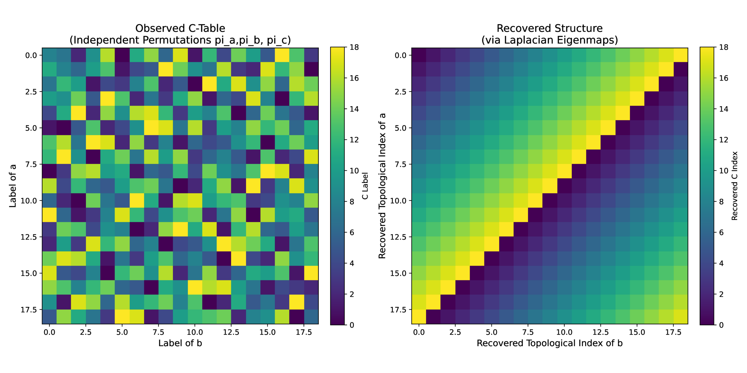
Starting with a task \(c = (a + b) \bmod (p)\) where \(p\) is prime, we need to infer an ordering of the integers \(a\), \(b\), and \(c\); in a MLP, we cannot use the communicative properties of addition, so need to rely on between-sample comparisons. This is possible with ‘experiments’: hold \(a\) constant and sweep \(b\), looking for matches in \(c\):

If \(c = c’\) then we know that \(b\) and \(b’\) are separated by \(\Delta = a_1 – a_2\):

and therefore must be neighbors. (\(\Delta \) is a ‘generator’ over the finite cyclical field \(p\)) Once you have an ordering for \(b\), you can infer a concordant mapping for \(c\) by simply holding \(a\) fixed. A similar construction works for \(a\), going back from (now ordered) \(c\) with a fixed \(b\). See cayley.py in the associated repo for an implementation and Figure 1 for a visualization.

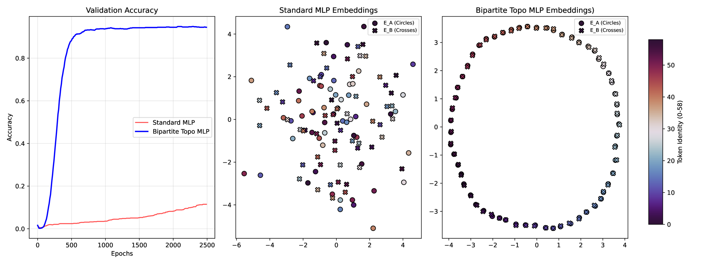
This approach can be applied to the encoding layer of an MLP by

1. Calculating the graph Laplacian based on proximity (adjacency per above)

2. Using the graph Laplacian matrix \(L\) to regularize the encoding \(W\) such that adjacent embeddings are similar¹¹ \(L = D – W\) where \(W\) is the adjacency matrix and \(D\) is the node degree; the square on the right, mesuring the \(L_2\) distance between embedding vectors \(w_i\) is completed after some algebra.:

   \[ topo\_loss = tr( W^T L W) = \sum _{i=0}^N \sum _{j=0}^N L_{ij} || w_i – w_j ||_2^2 \]

This works well, see topogrok.py and Figure 2

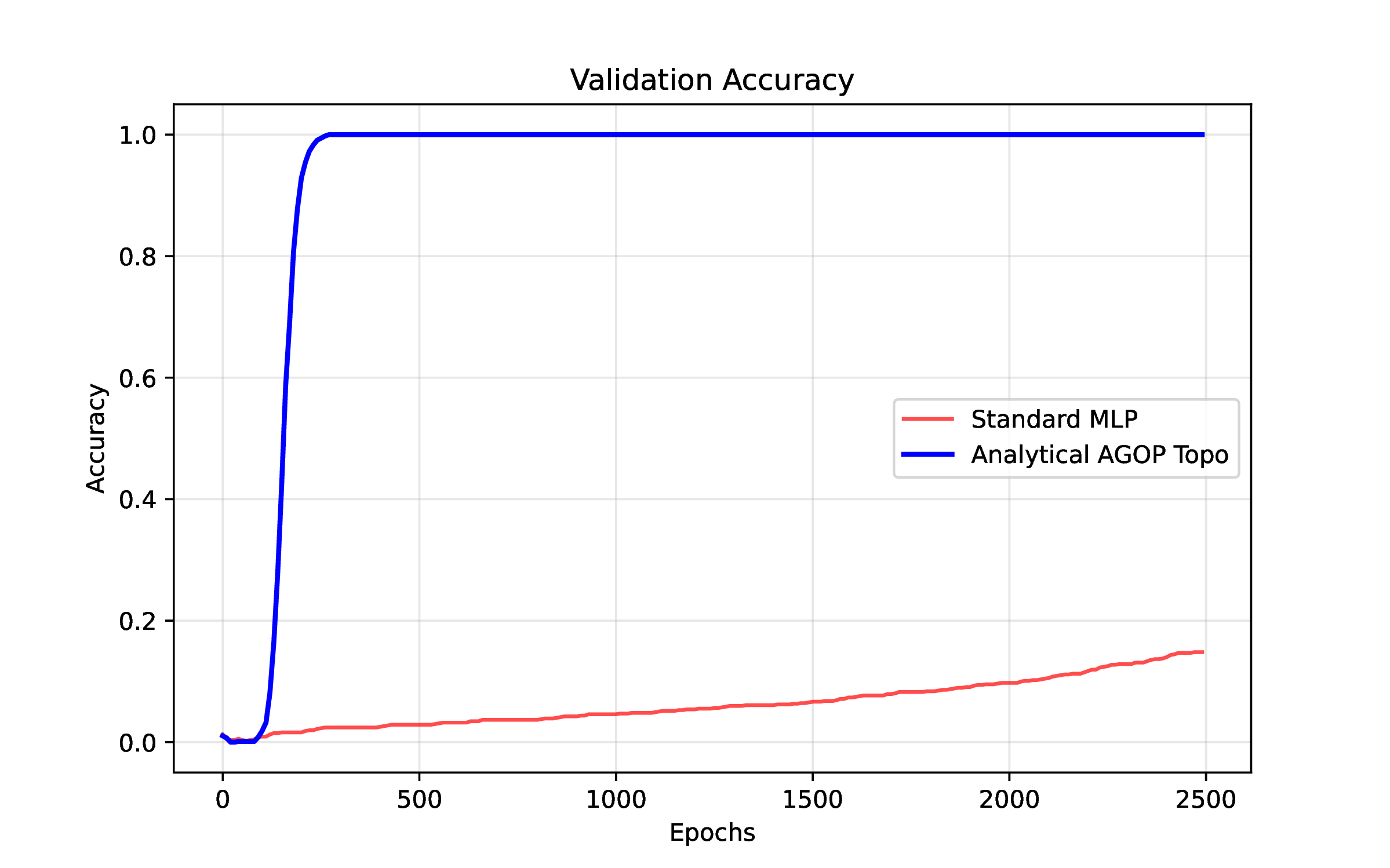
Another avenue for encouraging low-dimensional topology in network weights is to regularize the average gradient outer product (AGOP), which looks at (effectively) the correlation matrix of the gradient of the function (\(\frac {\partial output}{\partial input}\)) measured at the input points [2]. Minimizing the trace of the AGOP matrix in the input space is effectively a nuclear norm, forcing low-dimensional & ordered representations input encoding (here integers). See agopgrok.py and Figure 3

3 Transformers

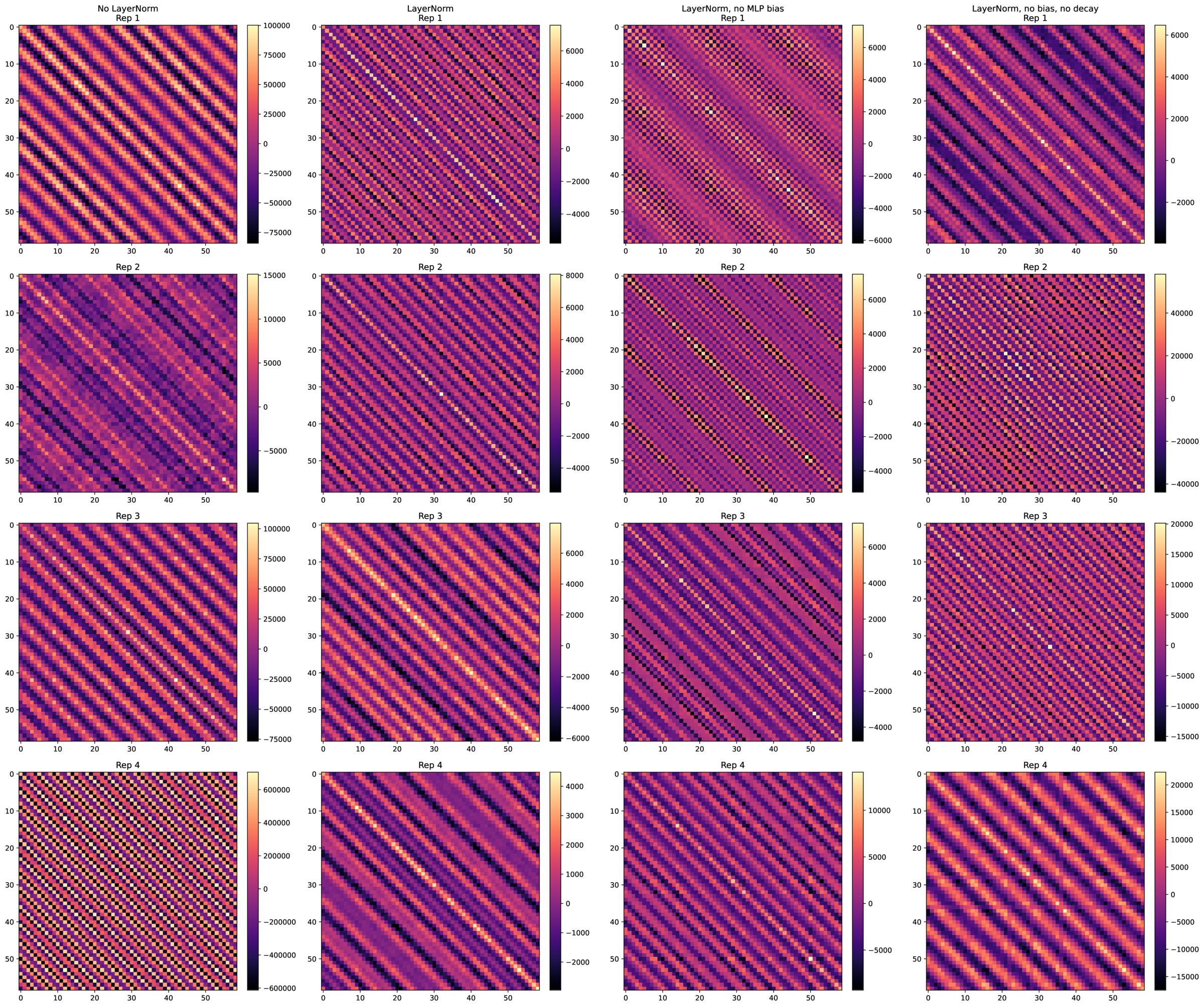
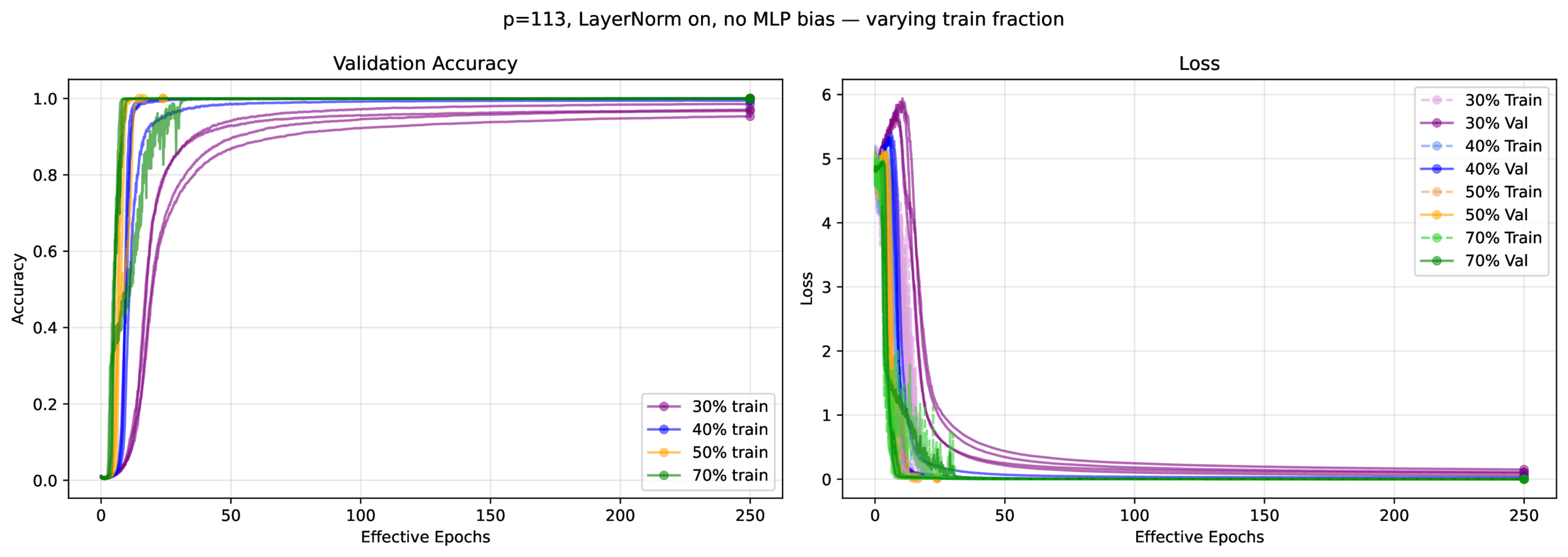
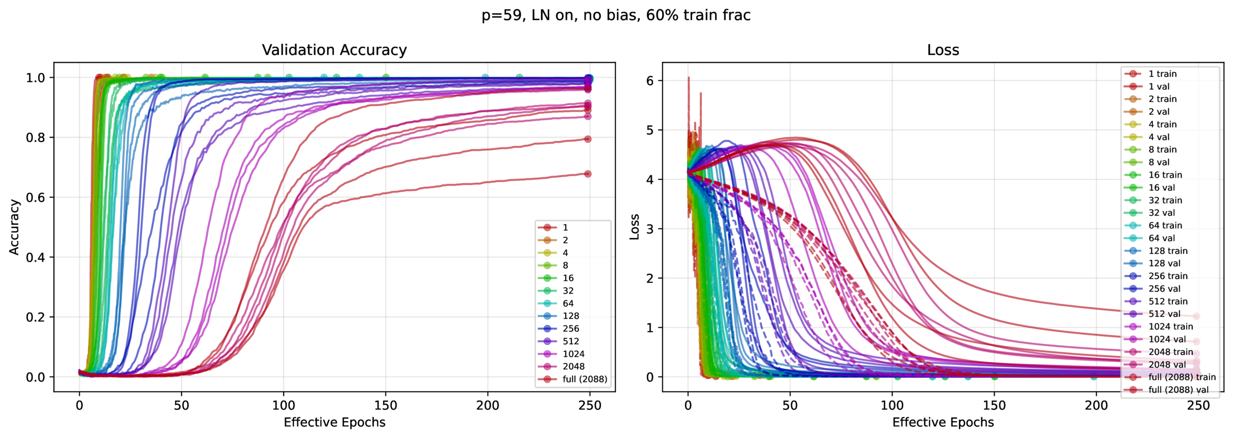
Now, does the AGOP regularization extend to transformers? It turns out not to matter, as transformers grok very quickly. This was surprising, as the literature suggests that you need thousands t otens of thousands of epochs to witness grokking. Instead, we found that you typically need \(\approx 30\) passes through the data. You don’t need \(L_2\) regularization (weight decay), or even layer norm; instead, what’s important is minibatch SGD (as well as training fraction, of course – can’t learn an ordering if there are no overlaps in \(a\), \(b\) and \(c\)).

We tried to replicate the configuration described in [1]: the model is a 1-layer, 1-head transformer, with a ReLU 4x expansion FFN layer, untied embedding and unembedding matrices, and either \(p=59\) or \(p=113\). See fastgrok.py for the implementation, and Figures 4 – 7.

4 Recap

What matters is:

• Minibatch SGD. With all else held constant, more gradient steps & less gradient averaging increases grokking speed, approximately linearly.
• Training fraction. A higher fraction increases the number of available measurable neighbors, each which constrain the representation, facilitating topology inference (apologies for not quantifying this).

Timothy Hanson

April 2026

References