Introduction
AI for constraint satisfaction problems is an important field researched for more than half a century. Sudoku, a puzzle where no row, column, or block can have two of the same number, is a popular benchmark to assess the ability of models to reason over constraints. With the rise of deep learning, many deep neural networks have been used to solve sudoku, such as transformers and graph neural networks. These networks perform well but are trained under supervision and assume access to a labelled dataset. Given the importance of identifying patterns in the structure of Sudoku solutions, these supervised methods may be limited in their capability to generalize to unseen puzzles (as combinatorially many exist) or perform well under limited data settings—and at the minimum, require a supervised dataset of initial puzzles \(x\) to final puzzle solutions \(y\).
Thus we instead employ an unsupervised generative modelling approach to learn the distribution of sudoku puzzles in hopes that our model learns moreso the structures and patterns of sudoku puzzles. Diffusion is a widely used generative model for all kinds of settings, and here we apply it to learn Sudoku puzzles. Since sudoku (a board that is a nine by nine matrix filled with numbers one through nine) is inherently a matrix of discrete numbers, we use a discrete diffusion model. While continous diffusion (such as the popular DDPM) can be used if sudoku boards are relaxed and represented in continuous space \(\mathbb {R}^{9\times 9}\), we believe that preserving the discrete nature of Sudoku puzzles is more natural and so opt for a discrete diffusion model.
Background
Diffusion at a very high level is a generative model defined by a forward markov chain (which “corrupts” the actual data distribution we care about to some prior distribution easy to sample from, such as complete noise); it aims to learn the reverse markov chain which can take a sample from the prior and progressively “decorrupt it” and transform it to a sample who comes from a distribution approximate to the actual data distribution we wish to learn. (For a more extensive treatment of diffusion models, Calvin Luo has a good tutorial (Luo 2022)).
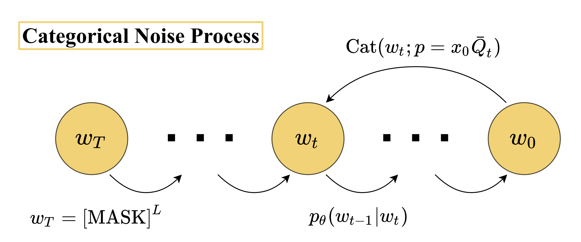
For discrete data, (Austin et al. 2021) introduce Discrete Denoising Diffusion Probabilistic Models. (For a more extensive treatment, please refer to their work “Structured Denoising Diffusion Models in Discrete State-Spaces”). A sequence \(\mathbf {x}_{t}\in \mathbb {Z}^{L}\) of \(L\) many discrete categorical variables of \(K\) categories \(x\in [K]\) has a forward corrupting markov chain defined by a transition kernel matrix \(Q_{t}\in \mathbb {R^{K\times K}}\). In the forward process, the transition kernel matrix \(Q_{t}\) is applied to all tokens or categorical variables in the sequence \(x_{t}\) independently (categorical variables are represented as one-hot vectors \(x\in \mathbb {Z}^{K}\)); thus for clarity we can just focus on the case where our sequence has one token \(L=1\) and we collapse to a single categorical variable \(x\). The one timestep forward transition probability of a categorical variable \(x\) is the categorical distribution induced by applying the kernel matrix to the previous state of \(x\); \(q(x_{t}|x_{t-1})=Cat(x_{t};p=x_{t-1}Q_{t})\) . Discrete Denoising Diffusion Probabilistic Models (D3PM) only work with discrete time markov chains; however, as seen later, more general continuous time diffusion models exist as well.

In the discrete time setting, the goal of diffusion is to learn the reverse transition process at each timestep, which is defined by \(p_{\theta }(x_{t-1}|x_{t})\). While this one step reverse transition can be directly modelled by a network, Austin et al. parameterize the one step transition through a denoiser \(\tilde {p}_{\theta }(\tilde {x_{0}}|x_{t})\):
where the denoiser is learned with a neural network. In brief this parametrization comes from applications of Bayes rule, where \(q(x_{t-1}|x_{t},\tilde {x_{0}})=\frac {q(x_{t}|x_{t-1},x_{0})q(x_{t-1}|x_{0})}{q(x_{t}|x_{0})}\) is derived using Bayes and we also have
where with our construction of the forward process we have \(q(x_{t}|\tilde {x}_{0})=Cat(x_{t};p=x_{0}\bar {Q}_{t})\) where \(\bar {Q}_{t}=\prod _{i=1}^{t}Q_{i}\) is the cumulative product of the absorbing transition kernels over time and we can also calculate (derivation is slightly involved) \(q(x_{t-1}|x_{t},x_{0})\) .
One thing that is important to note is that in the forward process, our transition kernel matrix \(Q_{t}\) is applied to each token in the sequence independently, meaning that each categorical variable forward diffuses independent of the other tokens. However, in the reverse diffusion process, this is not the case—our denoiser network \(\tilde {p}_{\theta }(\tilde {x_{0}}|x_{t})\) is a neural network that conditions on all tokens in the sequence \(\mathbf {x}_{t}=[x_{t}]_{l=1}^{L}.\)
This parameterization of a denoiser \(\tilde {p}_{\theta }(\tilde {x_{0}}|x_{t})\) allows for flexible calculation of transitions, such as skipping k-steps at once
Austin et al. consider various transition matrices \(Q_{t}\); we choose the simple absorbing transition kernel where a state transitions to absorbing state \([MASK]\) with probability \(\beta _{t}\), else stays the same. This simple transition kernel matrix allows for easy calculation of \(q(x_{t}|x_{0})=Cat(x_{t};p=x_{0}\bar {Q}_{t})\).
For the general transition kernel, we have as our diffusion loss objective for our denoiser \(\tilde {p}_{\theta }(\tilde {x_{0}}|x_{t})\) as
where the variational lower bound loss is defined as
Fortunately, Austin et al. conveniently show that the generative masked language model (MLM) objective (inferring the unmasked token of a masked token, as in the LLM BERT objective) is equivalent to our diffusion loss objective \(L_{\lambda }\) under the simple absorbing transition kernel. Thus it is enough for our model to infer the unmasked token of a masked token—and consequently it is enough for our loss function to simply be the cross entropy or log loss over the masked tokens.
Thus, we define the simple likelihood objective of predicting the unmasked tokens. With abuse of notation, we can simply write this as the cross entropy loss of predicting the actual unmasked sequences \(w_{0}\) drawn from our actual data distribution \(q(w_{0})\) given the masked sequences \(w_{t}\) drawn from the forward transition distribution \(p(w_{t}|w_{0})\):
More accurately, our cross entropy loss is calculated only over the tokens which are masked (say denoted by set of indices \(I\))
As usual we assume that our given dataset \(\{w_{0}\}\) is drawn i.i.d from the actual data distribution \(q(x_{0})\). To implement this loss in practice, our loss function is calculated over minibatches defined from the given training data \(\{w_{0}\}\); for each datapoint \(w_{0}\) in our minibatch we sample \(t\sim Unif\{[0,T\}\), our corrupted sequence \(w_{t}\sim q(x_{t}|x_{0},t)\), and then calculate an average of the cross entropy loss over the masked tokens.
MLM discrete diffusion for sudoku
To make the application of MLM discrete diffusion to sudoku concrete, we consider a dataset of sudoku solutions which we flatten row-wise into vectors \(\{w_{0}\in \mathbb {Z}^{81}\}\) containing tokens of digits one through nine. Then, using the MLM cross entropy objective above, we train our diffusion model, defined by a learned denoiser \(\tilde {p}_{\theta }(\tilde {w_{0}}|w_{t})\). Once our denoiser is learned, we can kick start the sudoku solution generation process by first drawing an initial sample \(w_{T}\) from the absorbing state prior (which is simply all [MASK] tokens) and then iteratively sample from the reverse transition probability
for each timestep \(t\in [T,1]\) to generate our datapoint \(\hat {w}_{0}.\)
This above process takes a completely informationless sequence of \([MASK]\) tokens and generates a (hopefully realistic and valid) sudoku solution; however, it is simply a sudoku solution. To generate solutions corresponding to some initial sudoku board \(x\), we use infilling generation. At each time step \(t\in [T,0]\) in the reverse process (including the prior sample), given some partially filled initial board \(x\) with non-empty cells/tokens with indices \(i\in I\) , we replace all tokens in the diffusion output \(w_{t}\) with indices \(i\in I\) to be the corresponding token in the initial board \(x\), or \(\forall i\in I\quad [w_{t}]_{i}:=[x]_{i}\). This ensures that our reverse generation process generates a sudoku solution conditioned on the given initial sudoku board.
Guiding MLM discrete diffusion models
Above we saw that we can train a MLM discrete diffusion model to learn the distribution of sudoku puzzles and also condition on a given initial board to generate a corresponding solution.
While this is reasonably performant, we can improve the output generation process by incorporating guidance from some relevant value function . In our case, we want to ensure that the solution satisfy the constraints of sudoku (no digit must be duplicated in any given row, column, or block) so we can incorporate some value function \(v(w)\) which scores how well a proposed solution satisfies the constraints. To get this value function in practice, given a dataset of some (partially incorrect) sudoku solutions and the number of row/column/block constraints violated, we can train a network in a supervised manner to predict how few constraints a given proposed sudoku solution violates.
The immediate challenge with incorporating a value function \(v(w)\) is that the value function might have a discrete domain: in our case, the value function scores a sudoku board \(w\) which is a sequence of discrete tokens. A discrete domain is not differentiable, which poses a question of how the value function signal would be incorporated in the diffusion generation process.
One workaround is to shift to a continuous domain rather than a discrete domain. For example one could embed all sudoku boards \(w\) not as discrete tokens but as real valued sequences \(w\in \mathbb {R}^{81}\). Alternately one could train a seperate value function that is defined not on discrete sequences \(w\) but rather some continuous hidden logits \(h\) corresponding to the discrete sequences. This is in fact what (Gruver et al. 2023) do with protein sequences: for any given (noisy) sequence \(w_{t}\) in the reverse diffusion process they take hidden states (which hidden layer is left as a choice parameter) \(h_{t}\) from a trained diffusion decoder \(\tilde {p}_{\theta }(\tilde {w_{0}}|w_{t})\) and then utilize a value function defined on the (noisy) hidden states \(v(h_{t})\) . Since by construction \(v\) is differentiable with continuous inputs \(h,\) we can take gradients of \(v(h)\) to guide the original logits \(h_{t}\) from the diffusion denoiser \(\tilde {p}_{\theta }(\tilde {w_{0}}|w_{t})\). However, this requires training a value function based on noisy hidden states and moroever requires the value function to be tied down to the outputs of one specific trained diffusion model \(\tilde {p}_{\theta }(\tilde {w}_{0}|w_{t})\).
In many settings, this assumption may not be applicable and we may only have access to a value function that is defined on the actual outputs: say a function \(v(w)\) that scores how constraint satisfying a given discrete sudoku board \(w\) is or as a more practical example a function \(f(p)\) which scores how correct a program \(p\) is.
To work around this, we can rely on the gumbel softmax trick, explained briefly below.
Gumbel Softmax Trick
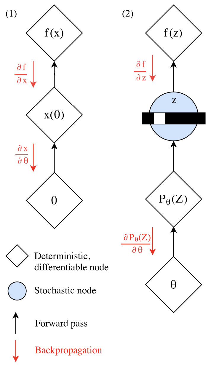
The Gumbel Softmax trick introduced by (Jang et al. 2017) allows for gradients to flow through a discrete or categorical variable.

In our case we want the gradients to flow with our setup \(h\to w\to v(w)\); \(w\sim Cat(\pi (h))\) is sampled from the categorical probability distribution \(\pi \) defined by logits \(h\) and then our value function \(v\) scores the discrete sample \(w\). The problem is that we have a discrete categorical sample \(w\) in the middle, which prevents calculation of \(\nabla _{h}w\) (and for that matter \(\nabla _{\pi }w)\) without any tricks. For simplicity let us now imagine that our sequence has length one: this means that our “sequence” is a categorical variable sampled from some probability distribution vector \(\pi \) with class probabilities \(\pi _{i}\). (In reality, with a sequence of length \(L,\) we would need a vector of class probabilities for each token in the sequence.)
More than half a century ago Gumbel proposed an efficient trick called the “Gumbel trick” to draw samples \(w\) from a categorical distribution defined by a vector of class probabilitites \(\pi \):
where \(g_{i}\) are i.i.d \(Gumbel(0,1)\) variables.
(Jang et al. 2017) introduces a continuous approximation of the argmax using softmax, explaining the name “Gumbel softmax trick”. As \(\tau \to 0,\) the vector \(y\) defined by
approaches the one-hot vector \(w\) defined by the argmax. This is a continuous relaxation and we see that our vector \(y\) ends up differentiable with respect to the probabilities \(\pi \), albeit being a continous vector rather than a discrete vector. With this approximation we now have a work around to approximate the gradient of our sample \(\nabla _{\pi }w\) using the approximation \(\nabla _{\pi }y\).
However, we do not need to keep our output \(y\) continuous. Similar to the straight through estimator, for the forward pass we can discretize our continuous \(y\) using argmax, leading to a desired discrete categorical variable \(w\) that can be passed to \(v(w)\); for the backpropagation step we can swap out the intractable \(\nabla _{\pi }w\) for our approximation \(\nabla _{\pi }y\).
Adding guidance in reverse process
Now that we can flow gradients from our constraint value function \(v(w)\) defined on sudoku board sequences\(,\) we can incorporate such gradients in our reverse sample generation process.
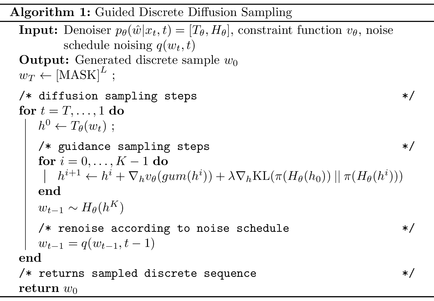
We do this by working in the logit space and guiding the initial logits from the diffusion denoiser \(\tilde {p}_{\theta }(\tilde {w_{0}}|w_{t})\). Naively, one might just simply add the gradient directly, such as \(h’=h+\nabla _{h}v(gum(h))\). However this poses a tradeoff between generating realistic samples faithful to the data distribution (coming from diffusion logits \(h\)) and generating samples which maximize the constraint value function \(v(w)\).
(Dathathri et al. 2020) in their work on plug and play language models handle this by regularizing the guided logits to the initial logits. Borrowing from this, our entire guided update step looks like
where \(i\) represents the update index and \(h^{0}\) are the initial logits.
Now at each reverse sampling timestep we update our logits with multiple regularized gradient ascent update steps. This leads the reverse process to bias towards final samples \(w_{0}\) that end up having a high constraint satisfaction score, leading to better solutions.
The entire sampling algorithm is shown in Figure 3.

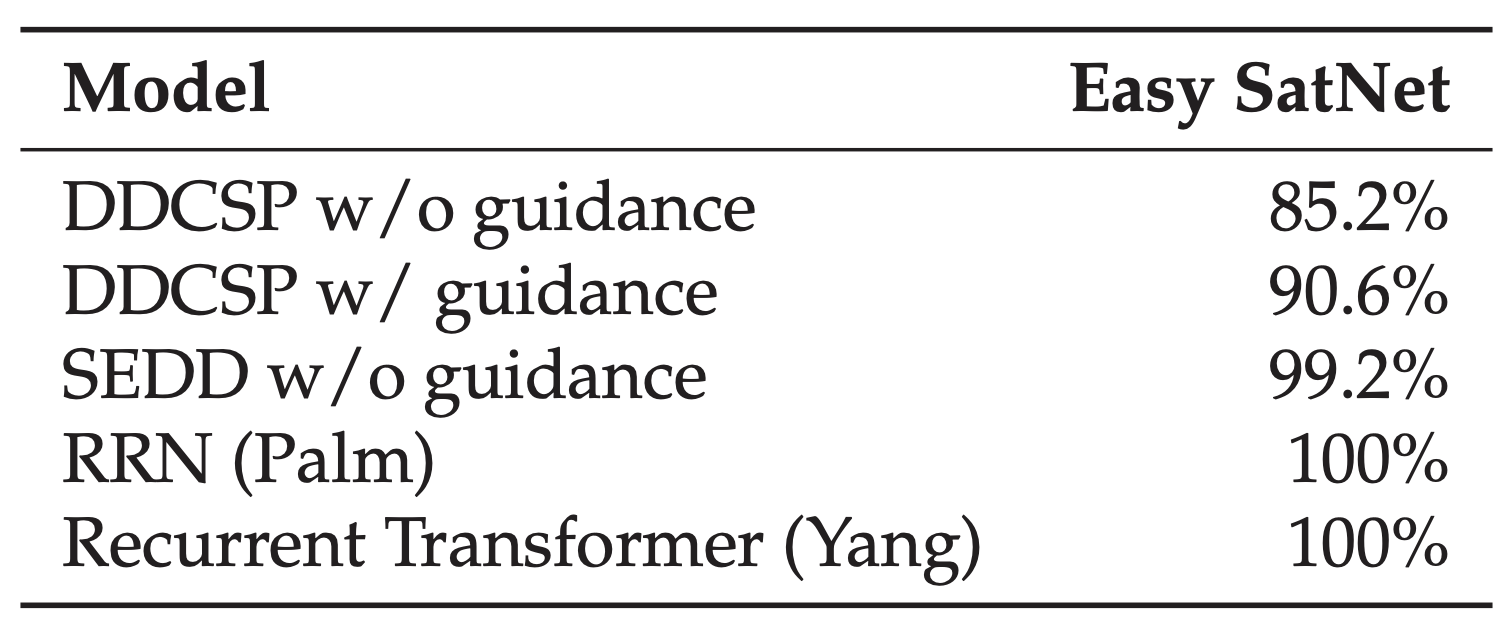
The impact of guidance on solve rate is shown in the results, Figure 4. We see that by adding constraint guidance we are able to increase the solve rate from 85.2% to 90.6%.
Score Entropy Discrete Diffusion
Score Entropy Discrete Diffusion (SEDD) introduced by (Lou et al. 2023) is a competitive, state of the art discrete diffusion model which outperforms similarly sized GPT models on perplexity scores. (An apt treatment on score entropy discrete diffusion models is out of the scope of this post, but for a introduction Lou’s blog post is a good starting point (Lou 2024)).
In comparison to previous diffusion models such as D3PM or the canonical DDPM, score entropy discrete diffusion is based on a continuous time markov chain.
Now, for some categorical variable \(x\in [K]\) with class probability mass vectors \(p\in \mathbb {R}^{K}\), we can characterize the probability distribution \(p\) evolving over continuous time, \(\{p_{t}\},\) using a differential equation rather than a bunch of discrete transition probabilities:
Here \(Q_{t}\in \mathbb {R}^{N\times N}\) is our diffusion matrix which evolve our probability vectors and define our forward markov chain. (Similar to our explanation of D3PM, we consider the case of only a single categorical variable: we will see why this is sufficient even when working with discrete sequences with many tokens later on.)
A neat result shows that with our forward continuous time markov chain given by \(Q_{t}\) there exists a corresponding reversal continuous time markov chain given by a reversal diffusion matrix \(\bar {Q_{t}}\):
where we can define our reversal matrix \(\bar {Q_{t}}\) in terms of the forward matrix \(Q_{t}\): \(\bar {Q}_{t}(y,x)=\frac {p_{t}(y)}{p_{t}(x)}Q_{t}(x,y)\) and \(\bar {Q}_{t}(x,x)=-\sum _{y\ne x}\bar {Q_{t}}(y,x)\).
In practice, we need to simulate the forward or reverse process and so for computational feasibility we use an approximation to this differential equation; in particular we consider a first order or linear Euler approximation and we have our approximate transition probabilities as
and
where both approximations are accurate up to error \(O(\Delta t^{2})\) and \(\delta \) represents the dirac-delta function.
Now given a defined forward process \(Q_{t}\), if we want to generate samples using the reverse process we can simply look at the reverse transition probability above and see that all we need is the ratio \(\frac {p_{t}(y)}{p_{t}(x)}\). At a high level what SEDD is doing is learning this ratio using a deep network, \(s_{\theta }(y)_{x}=\frac {p_{t}(y)}{p_{t}(x)}\), and then using this learned network in the reverse process simulation to generate samples.
Now in reality, we are dealing not with a single categorical variable but rather sequences \(\mathbf {x}\in \mathbb {Z}^{L}\) of many categorical variables. This significantly increases the number of all possible ratios \(s_{\theta }(\mathbf {y})_{\mathbf {x}}\) (in fact to exponential complexity). Thus for computational tractability, following (Campbell et al. 2022) they factorize the sequence and just have each token or categorical variable evolve independently of each other. Now, given that we are in a continuous time setting, the probability of two or more variables in a sequence evolving at same point in time \(t\) is zero: thus we only keep track of one token in the sequence transitioning for any time \(t\).
Notationally, with a sequence \(\mathbf {x}=(x^{1}…x^{L})\), we only need to keep track of some token with index \(i\) transitioning to some value \(\hat {x}_{i}\) and so our network only has to learn the ratio that differs by one token: \(s_{\theta }(\mathbf {x},t)_{i,\hat {x_{i}}}\approx \frac {p_{t}(x^{1}…\hat {x^{i}}…x^{L})}{p_{t}(x^{1}…x^{i}…x^{L})}\).
However, if we only change one token at each timestep, this means that for any given evolution most tokens will remain the same doing nothing and for long sequences \(L\gg 1\) our reverse process simulation will take a very long time to generate a final sequence sample. As a computational speed up, SEDD can employ tau-leaping, which is an approximation method to speed up sampling by essentially independently sampling each token in the sequence for each timestep.
With these tricks, SEDD is able to generate samples of high cardinality and dimensionality such as language sequences with reasonable computation.
SEDD for sudoku We train SEDD on sudoku board sequences \(w\) represented as sequences of categorical tokens as before. Given a trained SEDD network, to solve a given initial sudoku board, we again employ conditional infilling: in each timestep of the reverse sampling process, we replace the diffusion output to contain the non-empty initial sudoku tokens.
What we see in our results is that SEDD demonstrates state of the art sample efficiency on SATNet, a common Sudoku benchmark. Other models such as transformer or graph based supervised networks trained on SATNet also achieve 100% solve rate accuracy on SATNet and so SEDD is not any more competitive than typical supervised methods. However, it is notable that even with an order of magnitude less training data, learning from only hundreds of puzzle solutions (no supervised data needed) we get performant results.

Results

We demonstrate the results of our discrete diffusion model against some baselines. Palm is a graph neural network and Yang is a recurrent transformer, both trained with supervised datasets. DDCSP is the MLM discrete diffusion model. While DDCSP is not as performant as the supervised networks, we see that with guidance performance increases considerably. SEDD, the state of the art discrete diffusion model, is competitive with the supervised baselines.
Conclusion
In summary, we have shown how discrete diffusion models offer competitive performance on constraint satisfaction problems such as sudoku. By employing a guidance technique, we are able to further improve diffusion output solve rate. Moreover, we show that even with limited samples, state of the art discrete diffusion models exhibit performant behavior on sudoku benchmarks. A natural next step is to add guidance to the score entropy discrete diffusion process and see how guidance improves performance and sample efficiency.
Acknowledgements
I would like to thank Tim Hanson for reviewing this paper and providing feedback. This work was made possible through the philanthropic support of Schmidt Futures.
References
- Austin, J., Johnson, D. D., Ho, J., Tarlow, D., & van den Berg, R. (2021). Structured Denoising Diffusion Models in Discrete State-Spaces.
- Bansal, A., Chu, H-M., Schwarzschild, A., Sengupta, S., Goldblum, M., Geiping, J., & Goldstein, T. (2023). Universal Guidance for Diffusion Models.
- Campbell, A., Benton, J., De Bortoli, V., Rainforth, T., Deligiannidis, G., & Doucet, A. (2022). A Continuous Time Framework for Discrete Denoising Models.
- Dathathri, S., Madotto, A., Lan, J., Hung, J., Frank, E., Molino, P., Yosinski, J., & Liu, R. (2020). Plug and Play Language Models: A Simple Approach to Controlled Text Generation.
- Dhariwal, P., & Nichol, A. (2021). Diffusion models beat gans on image synthesis.
- Gruver, N., et al. (2023). Protein design with guided discrete diffusion.
- Ho, J., & Salimans, T. (2022). Classifier-Free Diffusion Guidance.
- Jang, E., Gu, S., & Poole, B. (2017). Categorical Reparameterization with Gumbel-Softmax.
- Lou, A., et al. (2023). Discrete diffusion modeling by estimating the ratios of the data distribution.
- Lou, A. (2024). Language Modeling by Estimating the Ratios of the Data Distribution.
- Luo, C. (2022). Understanding Diffusion Models: A Unified Perspective.
- Palm, R. B., Paquet, U., & Winther, O. (2018). Recurrent Relational Networks.
- Yang, Z., Ishay, A., & Lee, J. (2023). Learning to Solve Constraint Satisfaction Problems with Recurrent Transformer.