Deep learning models generalize surprisingly well despite being overparameterized. Traditional measures of capacity, such as VC-dimension or Rademacher complexity, suggest that overparameterization should lead to overfitting – but it usually doesn’t. Prominent explanations for this phenomenon include that stochastic gradient descent (SGD) selects ’lottery tickets’ from it’s weight initialization [1], that SGD learns smooth, low-order functions first [2, 3] or that SGD exhibits implicit biases favoring solutions with flat loss minima = better generalization [4, 5] (among others).
Here I propose here a complementary explanation based on the geometry of high-dimensional spaces: a network starts out as an undifferentiated, smooth and simple null model and moves toward complex differentiated models through a finite series of small steps. With overparameterization comes increased volume of the parameter space, but without change in the ability for small steps to make progress – hence the resulting models remain close to the null model, and thereby simple. (The idea does not explain phenomena like grokking or double-descent – just generalization with early stopping.)
This rather straightforward and obvious explanation is complementary to the neural tangent kernel; while it’s a perspective on something already known, it was a fun bit of experimentation & seems worth posting.
High-Dimensional Geometry and Hypothesis Space Volume
As the number of parameters & activations in a neural network increases, the total volume of the hypothesis space expands exponentially, with each additional parameter adding a degree of freedom, and each activation adding an axis of variation. This makes the network monotonically better able to model arbitrary data. However, it doesn’t – why?
- Boring Activations: Assuming that the internal activations of the network do not ”blow up” (a condition that is both necessary and desirable for stable training), both individual and layer activations start out all being similar due to the concentration of measure. The concentration of measure says that when a variable depends broadly on many others in a Lipshitz way – which is desirable in neural networks, to make them trainable – its value tends toward a constant. Rather than being \(\epsilon \)-orthogonal (as would be the expected consequence of the concentration of measure), this means that initial activation vectors are correlated, but not so much so as to be indistinguishable. See Figure 1. 11 This is directly related to the neural tangent kernel[6], where as the network width goes to \(\infty \), the activations become perfectly Gaussian A further wrinkle is imposed by normalization, like LayerNorm or BatchNorm. Since both these are smoothly-varying functions of their input, the concentration of measure applies to them; increasing the number of parameters decreases the variance of the normalization constant, which makes those initial activations look even more ’null’.
-
Constrained Optimization Dynamics: Gradient-based optimizers, such as SGD and Adam, navigate the weight space through small, finite steps. This itself limits the volume of parameter space they can access, with an additional restriction from the scalar loss. The scalar loss acts as a bottleneck for information about the direction and magnitude of updates.
At initialization, the activations in non-output layers of the network are similar, so separating them effectively requires the optimizer to make a series of directional ”nudges.” The nudges tend to be noisy due to techniques like dropout, intrinsic noise (or ambiguity) in the source data, and lack of meaningful differentiation of upstream layer tunings, which caps the signal-to-noise ratio of the loss-steps to \(b\) bits. Limited SNR means \(b\) is “small”, which limits the precision and direction of the weight updates.
Steps hence look a bit Brownian22 Or not at all stochastic, in the case of ‘pure’ gradient descent, limiting distance; from a volume perspective, the limited bits per loss evaluation caps partitioning of the space. Each partition can be thought of as a hyperplane perpendicular to the gradient update step, and the SNR of the step defines the soft-margin on the partition. Partitions hence slowly push the activations away from the starting null hypothesis.
An more nuanced perspective from the literature is that the network sequentially learns eigenmodes ?? or Fourier modes ??; the \(b\) bits per step are used to set the position on the eigenvectors or the Fourier coefficients.
Additional navigational constraints are introduced by algorithmic features of optimizers like weight decay, gradient clipping, and per-axis learning rate normalization33 Momentum may increase the volume by reducing the Brownian nature of the minibatch gradient steps.. Combined with batching (where a single scalar loss, of limited SNR, aggregates information from multiple data points), the total volume of hypothesis space that is practically accessible through optimization scales exponentially in the number of training steps (each step can partition the hypothesis volume by, ideally, \(b\) bits; overparameterization gets closer to this upper bound because in high-D spaces there are no ’dead ends’, only saddles), while it does not scale significantly with the number of parameters or activations. This is why early stopping works well.
Experiments
Cosine similarity
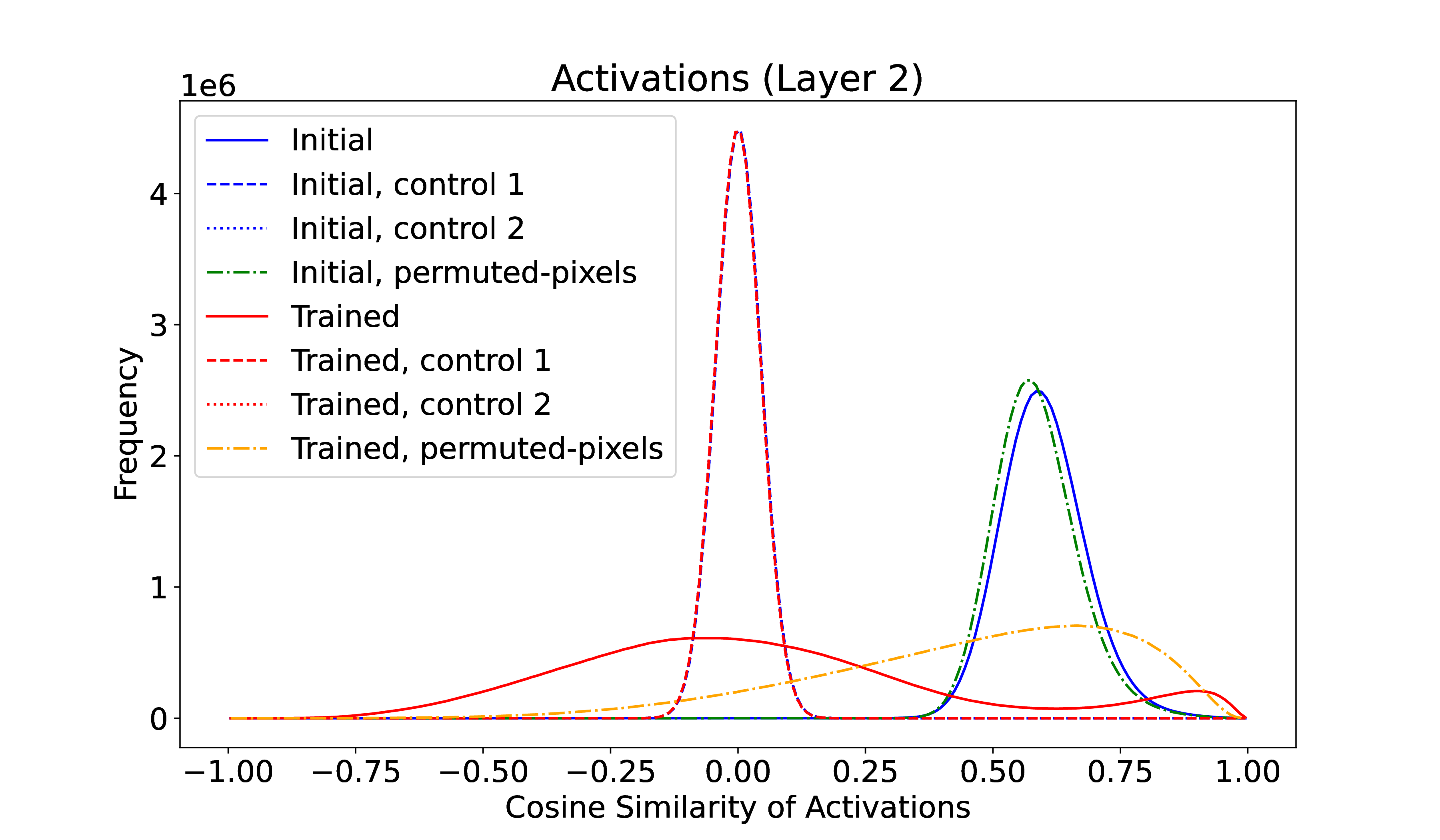
As a very preliminary and cursory test of the hypothesis, a small MNIST model (of course!) was trained. The model has 4 layers, with a ReLU nonlinearity between each, of size 784, 512, 512, 10. LayerNorm can optionally be enabled on the two hidden layers, and the optimizer was Adam (with or without weight decay). Activations in the penultimate layer (layer 2 in the figure – zero indexing) were recorded by running the 10k test set through the network before and after training for 10 epochs to \(\sim \) 98% accuracy. The similarity of these activation vectors was measured through the normalized dot-product aka cosine similarity44 I also experimented with normalized \(L_2\) distance; the results hold for this as well. As a control, the same activations were permuted per input datapoint (control 1) or replaced with Gaussian random numbers of the same mean and variance (control 2) before measuring the similarity. A further manipulation was to permute the pixel order of the input MNIST digits.
Figure 1 shows that even on this small network, the cosine similarity of the initial layer activations (blue) deviates very significantly from expected (controls 1 & 2). This initial similarity is nearly independent of input pixel permutation (dashed green), as expected for the untrained network.
Training the network decreases this correlation (solid red) to span more of the volume of activation space, and in the process pushing activations not in the training distribution to be more similar (dashed orange).
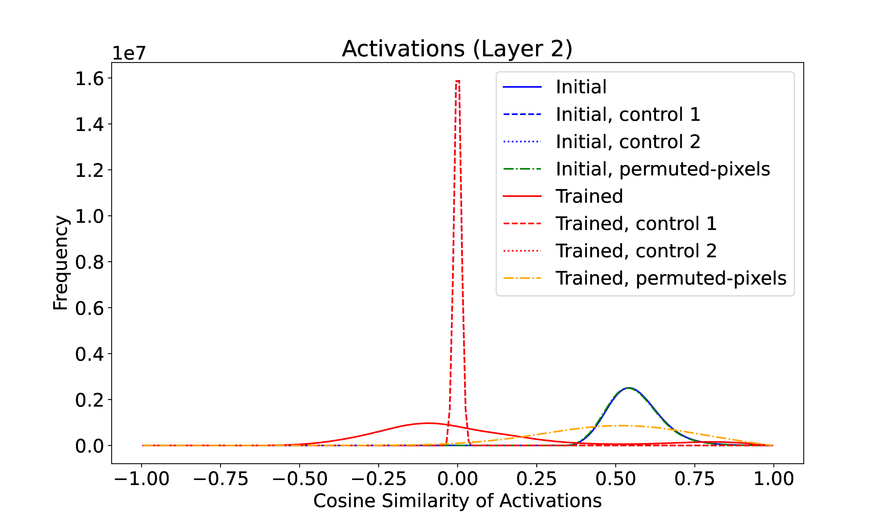
To test scaling, this experiment was repeated on a MLP size 784-8192-8192-10; all other parameters were unchanged. As expected from the concentration of measure, the control distributions become much narrower and more peaked – 8192-dimensional vectors are more \(\epsilon \)-orthogonal. Yet the initial distribution of activation similarities remains nearly the same! Initial activations between different test digits are quite similar, even in a very high dimensional space, and as with the smaller network, training expands their differences. See Figure 2.
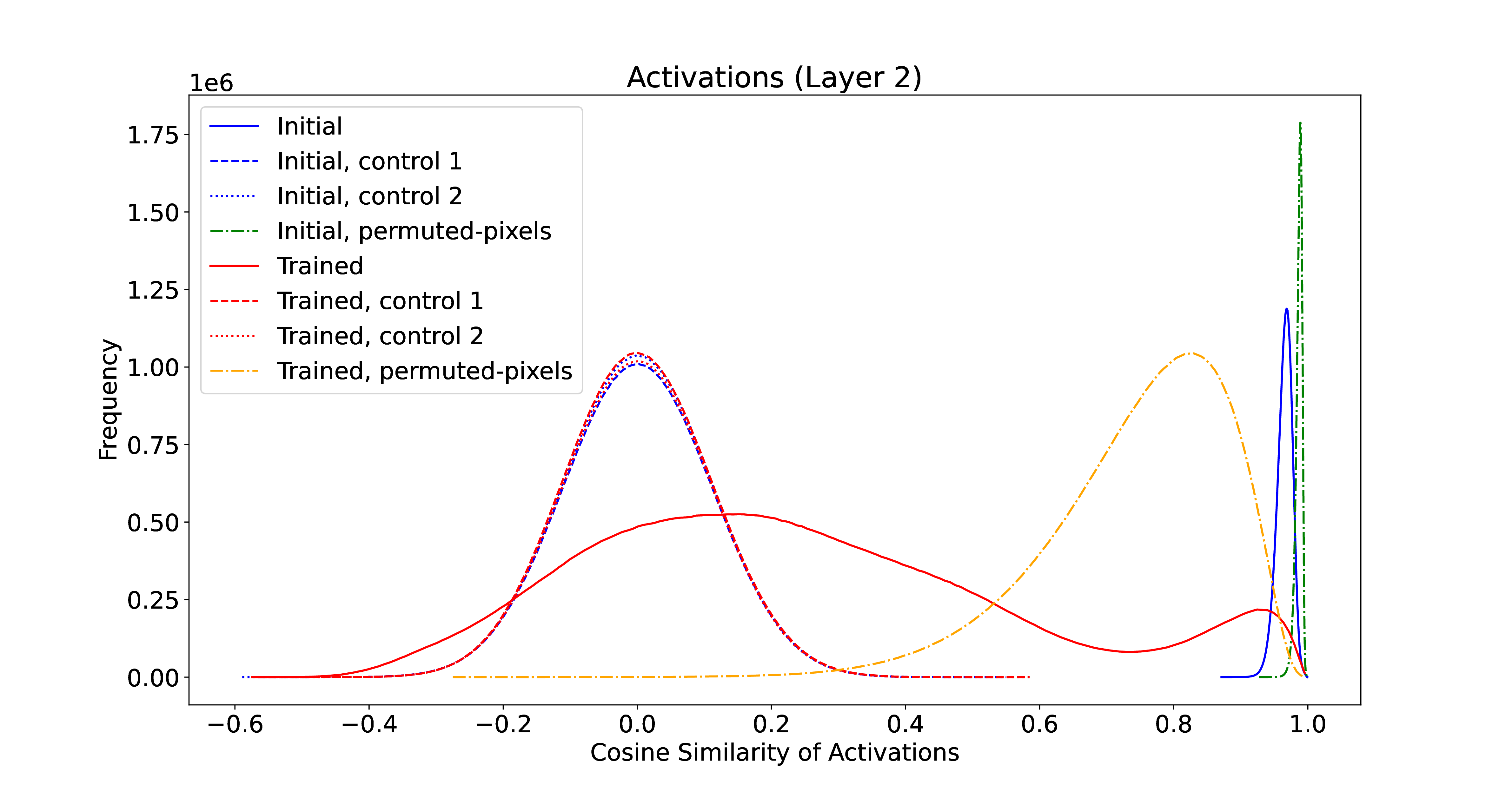
Finally, the same experiment was run on a LeNet-5 network. This resulted in even tighter clustering of initial activations. The convolutional structure of LeNet-5 restricts the hypothesis space (as desired), particularly restricting the starting or null hypotheses, which are all quite similar55 TBD if this is a general trend – have to try it out on transformers!. Training again expands this distribution.
Activation volume
Some effort was applied to validate the claim that the volume of activations increases with training. While this is trivially true – activations almost always grow in absolute magnitude with training – quantifying the change in volume is challenging in high dimensions (is the increase in volume meaningful?) 66 If you merely increase the activations, this is not interesting; If each of the activations is completely independent and interchangeable, this is also not interesting… quantifying this lies in the realm of mutual information, which is for another post.
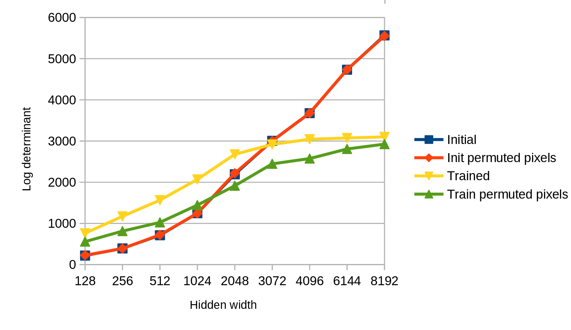
One first-order avenue is to approximate the distribution of activations as multivariate Gaussian & measure the volume through the determinant of the covariance matrix. As the empirical covariance matrix is biased to over-emphasize large eigenvalues, and under-emphasize small eigenvalues[7], instead the SVD of the activation matrix was taken, and the determinant was estimated from the clipped squared singular values, since if: \(A = U \Sigma V^T\) then \(cov = A^T A = V (\Sigma ^T \Sigma ) V^T\). Rather than taking the full expression for the volume of a multidimensional ellipse, we just use the log determinant, “LD”, as a metric.
| Hidden | Initial | Init ctrl | Init perm. | Trained | Train ctrl | Train perm. |
| 128 | 219 | 432 | 227 | 759 | 1372 | 557 |
| 256 | 392 | 866 | 389 | 1171 | 2689 | 812 |
| 512 | 712 | 1714 | 722 | 1564 | 5343 | 1024 |
| 1024 | 1247 | 3389 | 1242 | 2068 | 10497 | 1444 |
| 2048 | 2193 | 6605 | 2218 | 2679 | 20856 | 1914 |
| 3072 | 3005 | 9744 | 3001 | 2919 | 30699 | 2447 |
| 4096 | 3678 | 12750 | 3678 | 3045 | 40604 | 2575 |
| 6144 | 4733 | 18116 | 4737 | 3075 | 56511 | 2808 |
| 8192 | 5566 | 22233 | 5552 | 3101 | 66665 | 2925 |
What’s interesting is that the initial LD increases log-linearly with hidden dimension, as expected, while the trained LD saturates. With larger networks, the volume of activations goes down with training (at least as measured so coarsely). The control post-training (shuffled activations) continues to increase, suggesting that the activations are staying on a low-dimensional manifold within the progressively larger space. Interestingly, this effect persists without regularization! (\(L_2\) regularization decreases the asymptotic log determinant; increasing the number of epoch increases it, as expected.) SGD is not just limiting the volume explored – it is reducing the volume spanned by the activations. See Table 1 for more detail.
Implications for Generalization
The geometric effects work to impose a strong simplicity bias on overparameterized networks:
- Starting Simplicity: (1) implies that overparameterized networks begin their training journey in regions of the hypothesis space where solutions are minimally differentiated from the null hypothesis. Regardless of the network’s structure, activations and weights initially look ”the same.”
- Constrained Exploration: (2) suggests that the volume of hypothesis space navigable by the optimizer is small and concentrated near the start. Consequently, the reachable solutions are inherently simple and tend to generalize well, as they reflect minimal complexity relative to the vast hypothesis space77 As an aside, this is how most engineering proceeds as well – start simple and gradually elaborate. What’s missing from this analogy is refactoring or compression; regularization might be able to do this
This hypothesis also suggests that once away from the null hypothesis, it’s rather hard to navigate back toward simplicity. Distillation seems like a practical means of avoiding the limit, but further experiments with this & with regularization are required.
It also should be noted that small steps are but one way of moving around hypothesis space …
References
[1] J. Frankle and M. Carbin, “The Lottery Ticket Hypothesis: Finding Sparse, Trainable Neural Networks.” http://arxiv.org/abs/1803.03635
[2] N. Rahaman, A. Baratin, D. Arpit, F. Draxler, M. Lin, F. A. Hamprecht, Y. Bengio, and A. Courville, “On the Spectral Bias of Neural Networks.”
[3] Y. Cao, Z. Fang, Y. Wu, D.-X. Zhou, and Q. Gu. Towards Understanding the Spectral Bias of Deep Learning. http://arxiv.org/abs/1912.01198
[4] S. Hochreiter and J. Schmidhuber, “Flat Minima,” vol. 9, no. 1, pp. 1–42. https://direct.mit.edu/neco/article/9/1/1-42/6027
[5] S. L. Smith and Q. V. Le. A Bayesian Perspective on Generalization and Stochastic Gradient Descent. http://arxiv.org/abs/1710.06451
[6] A. Jacot, F. Gabriel, and C. Hongler. Neural Tangent Kernel: Convergence and Generalization in Neural Networks. http://arxiv.org/abs/1806.07572
[7] J.-H. Won, J. Lim, S.-J. Kim, and B. Rajaratnam, “Condition Number Regularized Covariance Estimation,” vol. 75, no. 3, pp. 427–450. https://www.ncbi.nlm.nih.gov/pmc/articles/PMC3667751/


