Sample efficiency, part 1: MLPs and Transformers

1 Introduction

After working on the classic CSP of Sudoku for several months¹¹ as of August 2024, we’ve figured out how to learn a ‘perfect’ model of the world – a model that can predict the legality and outcome of single actions entirely from observation. However, training is not per se efficient – for reliable model convergence, you need about 64k random actions, which takes several minutes to generate, and \(>\) 1hr of training on a single RTX 4090. When applying this world model to solve puzzles (entirely in imagination = planning), it still takes several seconds, even when accounting for efficiencies due to batched execution.

All this is quite a bit slower than a straightforward python implementation of backtracking search. Yet:

1. Backtracking search never learns from experience – the average time to solve a puzzle never decreases, which is both not desirable, and not what humans do.
2. On problems with action & state spaces larger than Sudoku, backtracking search won’t scale.

Human’s sample efficiency / ability to learn quickly + episodic and long-term memory enables us to detect patterns in both the board state and cognitive processing (chains of logical deduction) that enable dramatic search amortization and reduction of the space searched. Learning quickly involves inducing predictive models that both guide action selection (policies that decrease search breadth), and factorize the search space (decrease search depth – deductively avoid bad intermediate states).

2 Is deep learning sample efficient?

2.1 Model structure

This raises the vital question: is deep learning sufficiently sample efficient for bootstrapped active learning? That depends on the data, the optimizer, and the model.

Keeping the data and the optimizer fixed, let’s focus on model type. Deep learning provides (sometimes-implicit) assumptions about the data & how to process it into model structure. Roughly,

• MLPs assume vectoral data can be segmented by many hyperplanes, serially (layers) and in parallel (units).

  • This implies that the series of vectoral spaces are continuous along the depth dimension: points that are close have a similar mapping.
  • Generalization is therefore dependent on interpolation or regression working well for the data²² Not true for the phenomena of ‘grokking’, as discussed below..

• Convnets add to this that data is translation and scale invariant.

  • This forces all translations to map to similar activations: ‘close’ is preemptively collapsed.

• Transformers swap this invariance out with the assumption that all tokens are independent until proven otherwise. ³³ They also can have explicit limits on what tokens can predict ( = depend upon) others, e.g. causal masking.

  • This means that all computations are identical across tokens, and so variance and equivariance must be learned; rather than collapsing ‘close’, every token is by default treated similarly.
  • I.e. a transformer can learn {translation, rotation, scale} equivariance / invariance / symmetries.
  • This is contingent on supervised data ‘pulling’ out sub-spaces of the latent token space & finding small \(TC^0\) circuits for predicting these expansions[?].
  • Due to the structure of Softmax attention, the different \(TC^0\) circuits are not uniformly accessible by SGD⁴⁴ A corollary of them being compositional! This supposition is testable: if true, then the entropy of the Softmax on different layers almost never decreases during training, and so transformers like to learn ‘approximate automata’[1] based on the vagaries of the data and initial conditions.

This abbreviated sequence of models goes from having the minimal assumption of smoothness, to building in the ability to represent symmetries. We will look at MLPs first before moving to transformers.

2.2 MLPs

Rather than asking if MLPs are sample efficient, it’s productive to instead ask if nominally higher capacity models are more likely to overfit the data. If they do overfit, this then the high-dimensional mapping is not smooth and does not well interpolate & generalize the data. If they do not overfit, independent of the number of parameters, even while the train loss goes to \(\approx 0\), then all the datapoints are recorded and interpolated within the limits of the model assumptions \(\rightarrow \) the model is sample efficient. Sample inefficiency meanwhile may come from regularization: data provided to the model is not exactly learned, which may be caused by with dropout, \(L_1\) / \(L_2\) weight or activation regularization, or other smoothness constraints.

– –

All DL uses continuous parameterization, so that in addition to the statistics in the optimizer, there is fixed memory⁵⁵ Many other optimizers (e.g. backtracking search) have variable and expanding memory that increases with task complexity (e.g. tree depth) during the optimization process. Due to this fixed memory, and because a priori you do not know the complexity or expressivity of the model to be fit, there is an emphasis on overparameterization, sometimes with more parameters than the training data ⁶⁶ Overparameterization makes more complex models accessible and also helps trajectories escape of local minima.

This overparameterization makes many statisticians uncomfortable, since it also increases the model capacity, and so would also increase the risk of overfitting. This turns out not to be true, which we can illustrate by comparing two networks:

1. A network that’s initialized with small random weights, aka Xavier initialization.
2. A network that’s initialized with all zeros, and individual neurons ’turn on’ to capture parts of the error stream. This allows the network to explicitly allocate capacity gradually.

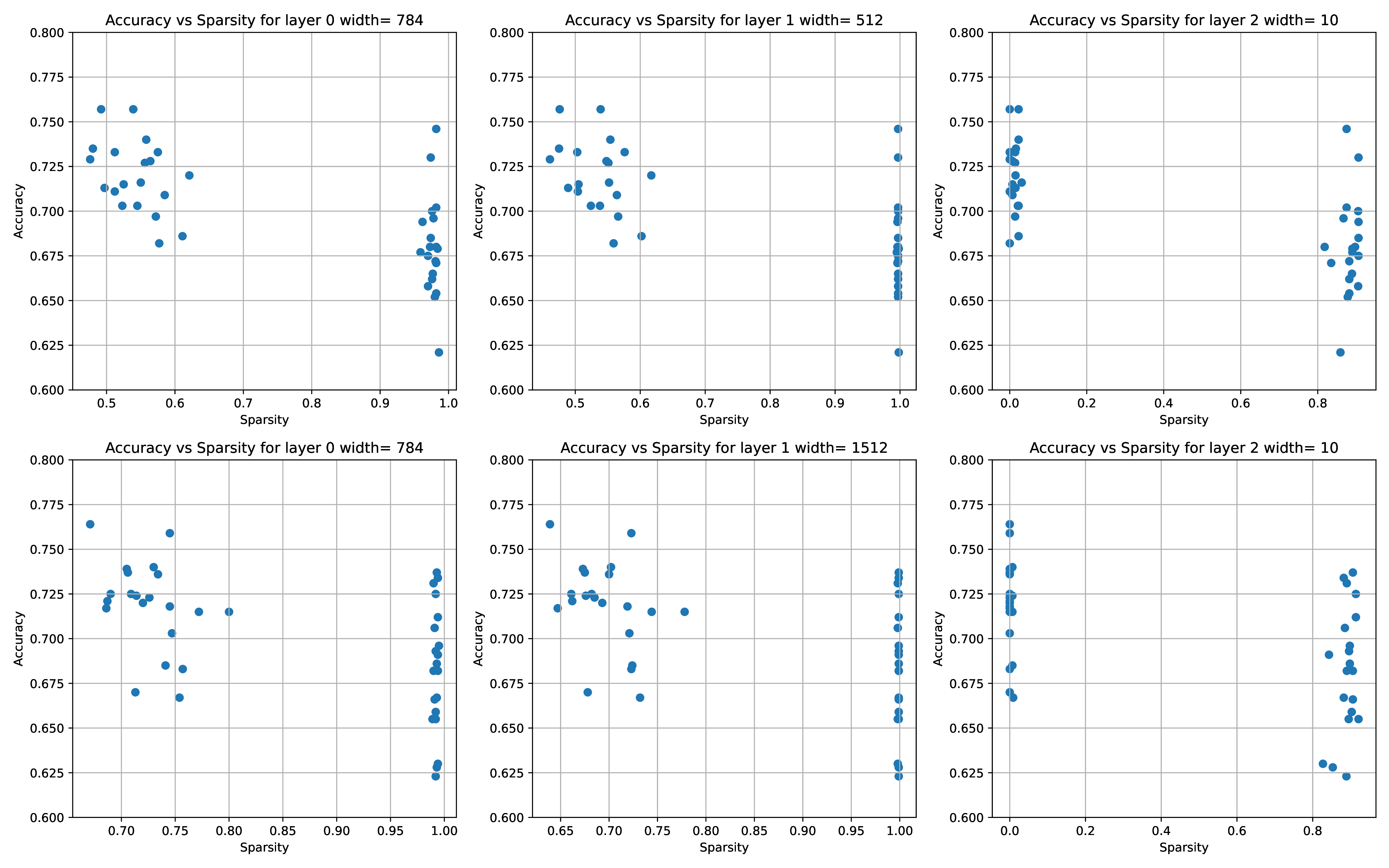
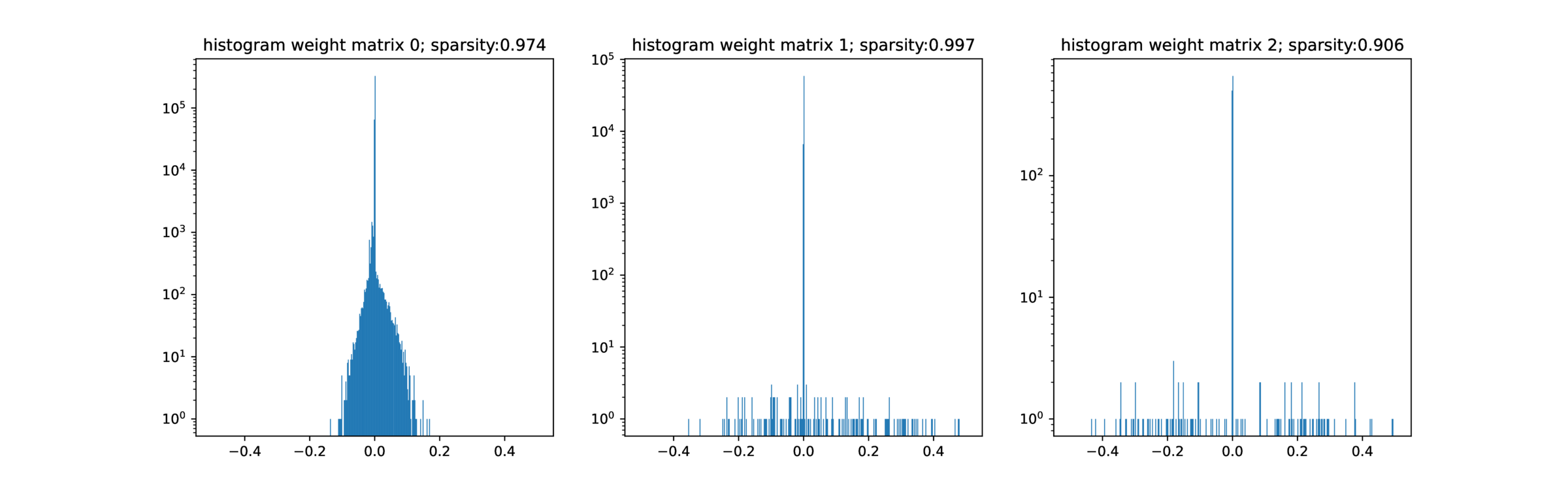
The 3-layer MLP networks are trained on that old standby, MNIST, only we experiment with 100 training points and 69900 test points, and assess models on their classification accuracy, where a random model gets \(\sim 10\%\) correct.

As shown in Figure 1, SGD can on average find a better-generalizing solution when the network is initialized with small random weights; aggressive sparsification has no positive effect, suggesting that the raw number of non-zero parameters has little effect on overfitting⁷⁷ Of course, this is not a perfect comparison – the selection of which parameters to make non-zero is still drawn from high dimensions – but the description length of the sparse model should be much lower. ‘Should’ because the overparameterized non-sparse model is likely much less sensitive to parameter noise, and so quantization to reduce the description length should affect performance less, as seen in LLMs.

This is rather surprising from a Bayesian perspective: adding more parameters to the model should make the total number of models grow exponentially, hence making any given model a posteriori less likely – and more likely to overfit the data and not generalize. This is not what we and countless others have seen. A working hypothesis is that instead of starting with exponential number of models, and using optimization to select from them, requiring concomitant quantities of data⁸⁸ Similar to the lottery ticket hypothesis, you instead start with all models being essentially equivalent and statistically indistinguishable.

SGD & friends add structure to the models by expanding the probability volume of model behavior. Specifically, SGD allocates state (neuron activations) dynamically, at the same it differentiates the weight matrix. See this post for more. The initial assumption that ‘all hyperplanes are nearly flat’ means that all input and hidden dimensions are assumed equivalent until proven otherwise, which means that all models initially behave \(\approx \) equivalently. The sparsity results indicate that it does not matter much if the directions of those hyperplanes is axis-aligned (at least, for MNIST). ⁹⁹ Compare with Anthropic’s superposition results A further surprise is that, within a broad regime, both Adam and AdamW never seem to overfit (i.e. train loss goes to zero yet test loss blows up.)¹⁰¹⁰ But … why would they push on probability volume where there is no data support?

In terms of interpreting raw sensory data, the baseline performance of MLPs is strong: \(> 70\%\) performance on MNIST-100 is quite good! Despite the allocation arguments above, I think there is a far simpler reason that properly designed MLPs don’t overfit: they are only continuous mappings, with no expansive internal state.

2.3 Transformers

No internal state is not true of transformers, which have state (the attention matrices) that’s outside an affine transformation of the input data. Adding this state makes the model more expressive and more capable of supporting concise relational algorithms, but also makes it also more prone to overfitting [3]. This happens gradually: as the models get larger, the means for SGD to push on probability volume is no longer is well aligned with the computations required to solve the task, and you do get overfitting.

¹¹¹¹ This suggests a straightforward means of improving the generalization quality of transformers: (1) Adjust the weights so that all layers and attention matrices are scaled to be approximately similar, conditional input data. This is a necessary compromise, as activations must be distinguishable via SGD, but not so much to be distinguishable by downstream layers. Tricky! (2) Use multiple Softmax calculations so that, on average, they are the same – but can be differentiated by SGD.

At very large scales, it would appear that transformers are sample efficient – LLMs famously can do ‘zero shot’ learning. Yet, as argued in a previous blog post, this is merely reflecting their learning of (approximate) programs from structure in the training data. Programs are by nature generative, so LLMs do generalize well, but it does not mean that the model itself is sample efficient. Rather it has learned to copy the reasoning-structure of the dataset; as the training datasets are huge and have redundant structure for common motifs, there is minimal restraint on sample efficiency.

As mentioned above, transformers assume that all tokens are uniformly (in)dependent, but the models are biased toward discrete and one or few-hot relations through the Softmax on the attention matrix. This is reflective of the sparse causal structure of the world, and especially our linguistic world, but it does seem to require significant data to whittle down which-of-N tokens is predictive of the N+1 token. Learning the attention matrix is effectively inferring a parse-graph over tokens, with priors and limitations of what that graph may be. In comparison to MLPs, overfitting is a natural behavior of a transformer that is not sufficiently constrained: it can drive the attention matrix form spurious correlations in the data.

E.g. there is something like \(\sum _{i=1}^{n} w_i {n \choose i}\) different ways of arranging attention form a context of \(n\) to one token, where \(w_i\) is the softmax weighting for the number of active & predictive predecessor tokens, and \(\sum _{i=1}^{n} w_i = 1\). Parallel training constrains this¹²¹² IID training may disrupt this (a curriculum would be better), but still that’s a lot of different potential models!

To demonstrate this, we have experimented with a toy test problem, ‘setfind’. The goal of setfind is to locate a statically-tagged (over the learning task) member of a set, retrieve its information, and do a simple operation on this information¹³¹³ This operation is essential to increase the number of combinations & keep the model from simply memorizing the dataset. See the Appendix for an experiment that omit this operation. Here a transformer is supplied with a list of tokens (a set), one of which is a ‘cursor’ token, and the rest which are input tokens or ‘distractor’ tokens. The task is to predict the distance between the cursor token and the zero token, as measured via a positional encoding. The order of all tokens, inclusive the cursor token, are randomly permuted. The signed distance is provided as a supervised learning signal.

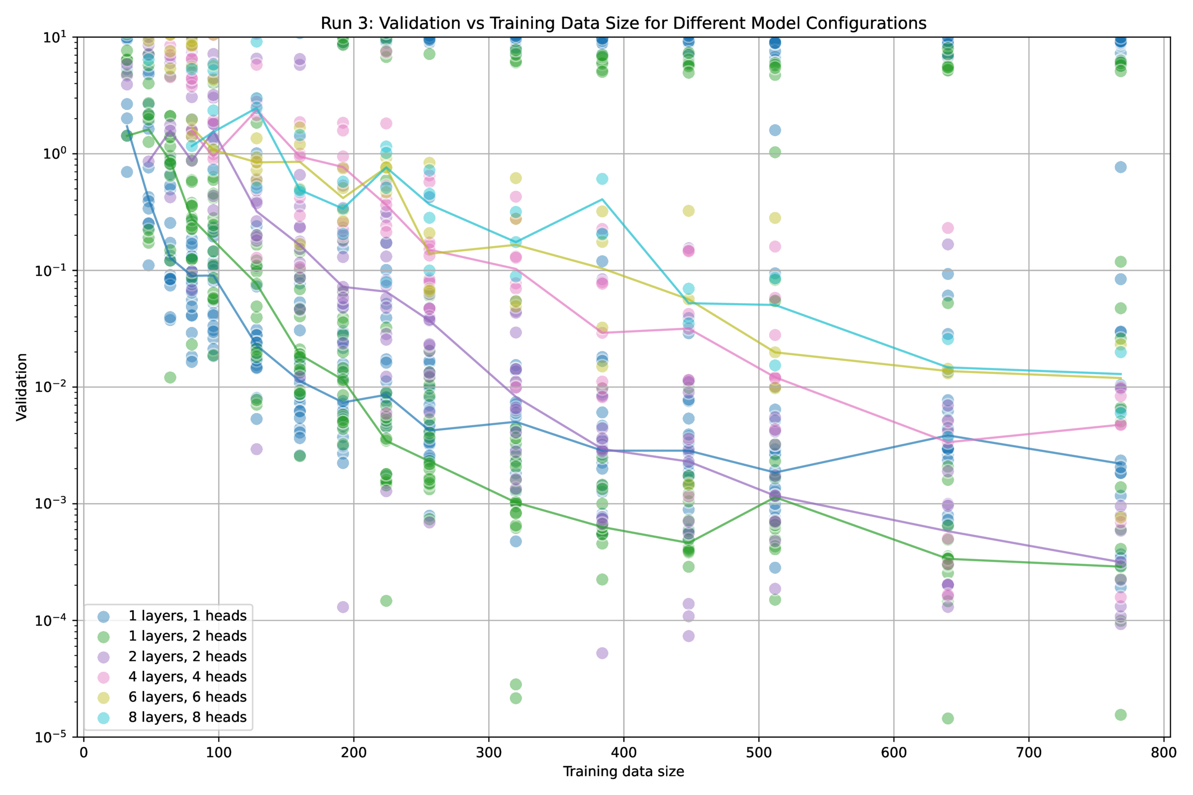
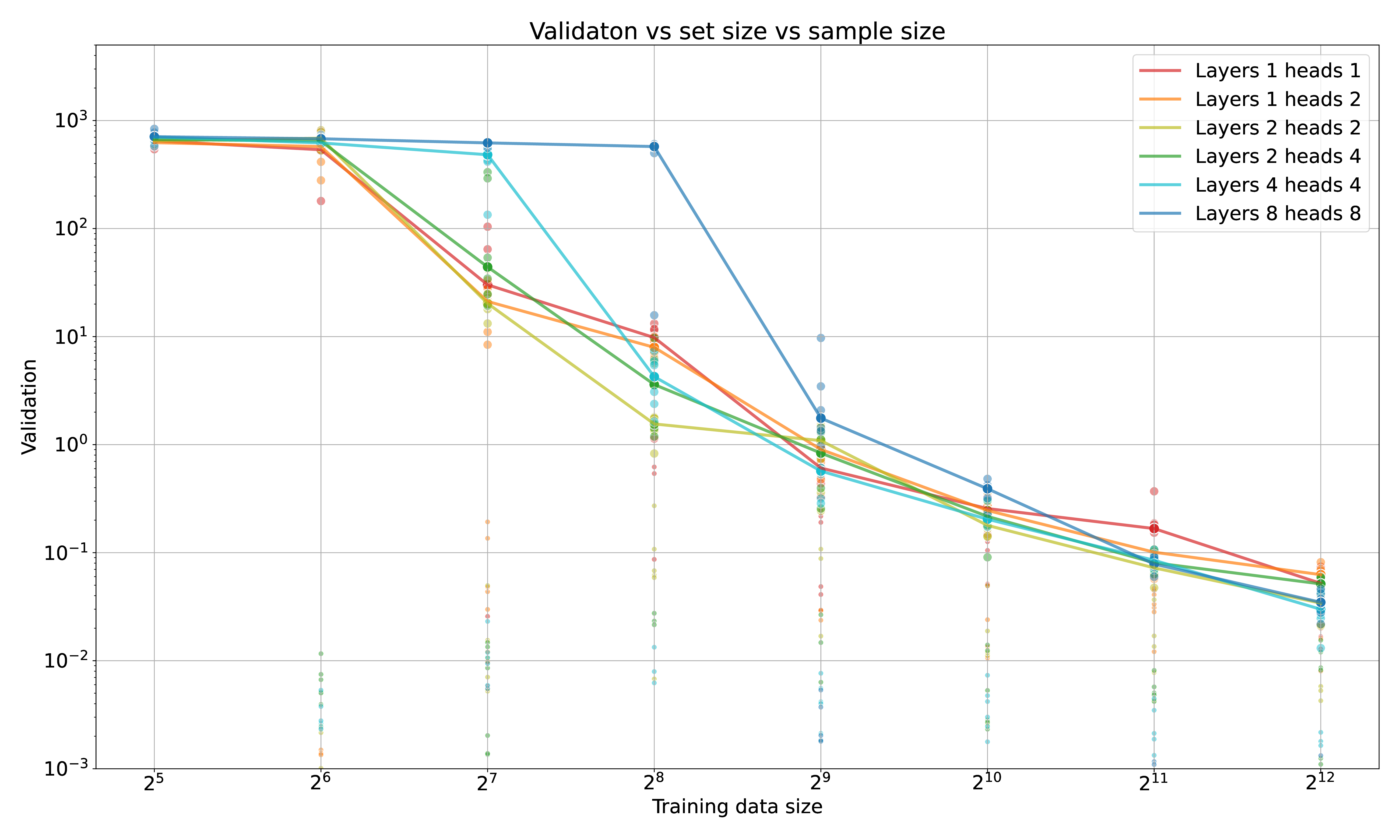
This problem is equivalent to learning a single ’hard’ linkage to one-of-n elements in a set – a basic operation of dependency-creation. As consistent with a Bayesian perspective, sample efficiency scales with model size on this problem; see Figure 2. As you increase the complexity of the model, the data required to solve the task increases – somewhat gracefully, but monotonically.

This gets back to the double-edged sword (box above): adding more model capacity (through layers + heads \(\rightarrow \) attention matrices, not parameters) increases the available state, hence model capacity, hence the probability that SGD finds a model not in the equivalence class as the actual data-generating process. This could be addressed by making the search discrete: training multiple models and comparing test losses, which is the straightforward way of making larger capacity models inaccessible to SGD. If larger-capacity models are accessible to SGD, then there is a chance that it will erroneously find the wrong causal structure; this probability must increase monotonically with increasing model capacity. The converse is illustrative: if it does not increase with model capacity, then necessarily higher capacity models are not accessible.

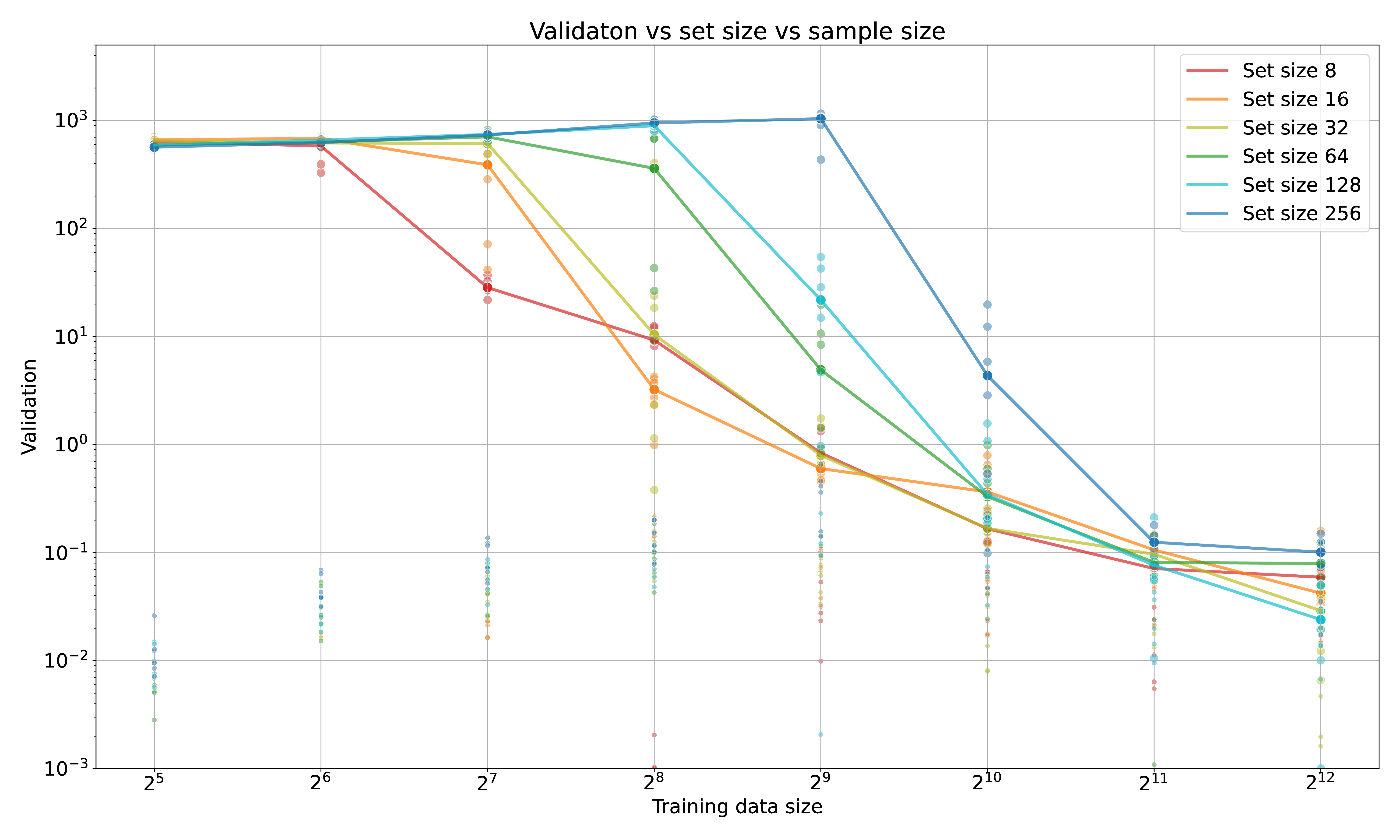
Sample efficiency also depends on \(n\) – the size of the set to be selected from. If the set is ordered, then the optimal strategy is binary search, where the correct element can be found in \(log_2(n)\) steps. This is not the case with a naïve transformer, which has no knowledge of the ordering of the set elements (even though they are given ordered positional encoding!) – on average, a model requires \(4n\) – \(8n\) batches. As each batch is a full example set (as described above), this means it needs \(> 4n^2\) set elements or ‘tokens’ to solve a one-of-\(n\) selection task. See Figure 3.

This is a contrived example, but still illustrative that (without help) transformers are not natively sample-efficient at figuring out which token to attend to. There are likely workarounds leveraged by frontier LLMS:

• Selection problems with large \(N\) are broken down into a series of smaller problems, which can be learned sequentially. Dividing the task into two problems reduces the sample requirement linearly, by a factor of 2. These ‘breadcrumbs of thought and factorization’ are prevalent in the human-generated data, since we also have to solve the same problems!
• The model learns semantic as well as grammatical, syntactic or other ‘type’ information, since it has to predict both; just like a type system benefits programming, so to can it constrain token-search in a transformer.
• The model does learn an ordering over elements, which makes causality-search look much more like a \(log_2(N)\) process¹⁴¹⁴ Which suggests a follow-up experiment: grokking \(\times \) setfind. I think this is consistent with, among other things, the effectiveness of RLHF / RLVR, but would require the emergent coordination of many heads within the transformer. Anecdotally, dot-product attention is not fundamentally ordered.

In the ‘setfind’ experiments above an additional wrinkle is that adding distractor dimensions to the latent vector decreases sample efficiency and increases the probability of non-convergence. Distractors in this case are axes of variation that do not correlate with the task; such a situation could be encountered in the first phases of training, or when there are many different meanings to words & tokens …

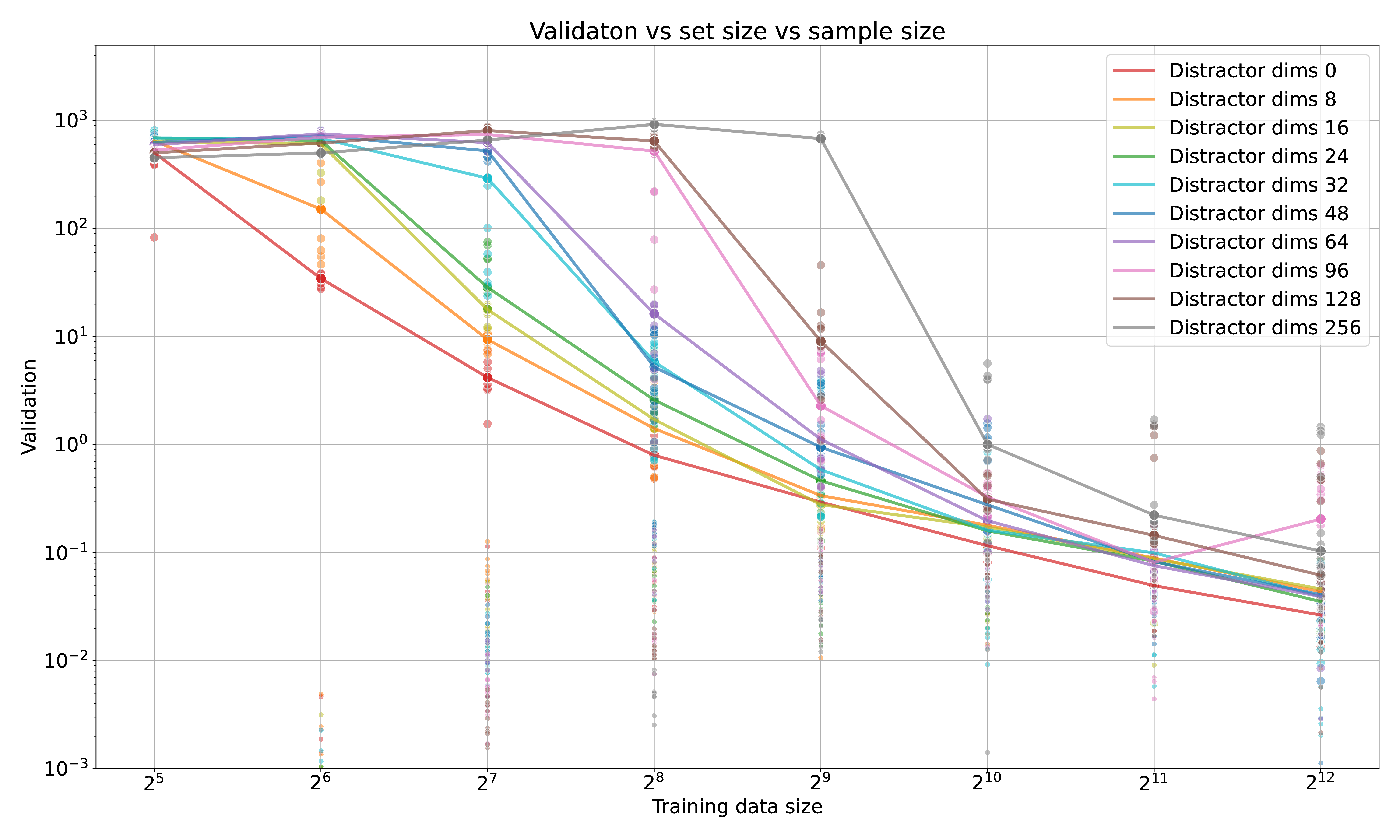
A core component of the transformer architecture is the MLP layers, which operate on the data within a token, dependent only on the source and destination token – a transformer is something like a message-passing network. Per Figure 2, it seems that these MLP layers gracefully degrade from the curse of dimensionality, as in the MNIST-100 experiments – but I do not think there are any shortcuts to inferring the dependency map by setting the Q and K matrices. Indeed, adding distractor dimensions to the latent dims decreases performance and increases the data requirement¹⁵¹⁵ Distractors could mean making a transformer do many things at once – which, perhaps, is not what LLMs are doing since they are trying to emulate human thought, and we tend to think in terms of fairly constrained Markov blankets.

3 Concluding thoughts

There are many more model architectures and types than just MLPs and Transformers, of course. State-space models, convnets, U-nets, RNNs like LSTM or GLUs, VAEs, VQ-VAEs, diffusion models, ¹⁶¹⁶ which is more of a training-inference paradigm than an architecture, energy-based models, G-flow nets, etc. all work to learn and model particular types of data. Yet transformers and seem to posses a degree of universality¹⁷¹⁷ E.g. you can remove the convolutional layers from a ViT and improve performance [4], even if they are sample-inefficient, as shown here. What is being computed and learned in their attention matrices? How do these inferred dependencies between tokens and additional state bear on modelling data? We will delve into these issues, and how transformers and other models can be be made more sample efficient, in a future article.

This post investigates the sample efficiency of MLPs and transformers and finds that the former tends to efficient (given enough compute), while the latter suffers from having excess accessible internal state. A future blog post in will look more broadly at model architecture-structure and optimizer form-function from the lens of model induction, and investigate how they relate to sample efficiency.

4 Appendix

References